Gradient Forest
Environment Agency
05 December, 2025
CaseStudy5.RmdIntroduction
This case study outlines a hydroecological modelling approach to explore the response of diatom community composition to flow and other environmental variables. It uses a nonlinear method designed to detect thresholds in species abundance patterns called gradient forest analysis (Ellis et al., 2012), using a subset of the Environment Agency’s National Drought Monitoring Network (NDMN) sites, as used in the HE Toolkit Vignette.
Other elements of this case study include illustrating the typical workflow involved in processing and harmonising species abundance data, and the importing and processing of additional environmental data on catchment land use. It is optimised for viewing in Chrome.
Set-up
Install and load the HE Toolkit:
#install.packages("remotes")
library(remotes)
# Conditionally install hetoolkit from github
if ("hetoolkit" %in% installed.packages() == FALSE) {
remotes::install_github("APEM-LTD/hetoolkit")
}
library(hetoolkit)Install and load the other packages necessary for this case study:
if(!require(pacman)) install.packages("pacman")
pacman::p_load(knitr, DT, kableExtra, htmlTable) # for tables
pacman::p_load(geojsonio, leaflet, rmapshaper, sf) # for maps
pacman::p_load(remotes, insight, RCurl, patchwork, rnrfa, vegan) # misc
pacman::p_load(dplyr, tidyr, lubridate, stringr, magrittr, tibble) # tidyverse
library(ggplot2) # plotting
# Conditionally install gradientForest from github
if ("gradientForest" %in% installed.packages() == FALSE) {
install.packages("gradientForest", repos="http://R-Forge.R-project.org")
}
library(gradientForest)
## Set ggplot theme
theme_set(theme_bw()) Metadata file
We load the same metadata file as used in the vignette, containing a lookup table of site IDs for the sites in the NDMN.
# load master file
data("master_file")
# make all columns character vectors
master_file$biol_site_id <- as.character(master_file$biol_site_id)
master_file$rhs_survey_id <- as.character(master_file$rhs_survey_id)
# Get site lists, for use with functions
cs5_biolsites <- master_file$biol_site_id
cs5_rhssurveys <- master_file$rhs_survey_idDiatom data
Import data
As there is currently no bespoke function in the HE Toolkit to import diatom data we instead download diatom data ‘en masse’ from the Ecology Data Explorer (EDE) bulk downloads page (https://environment.data.gov.uk/ecology/explorer/downloads/), and unzip and save the folder locally. We then import and filter the data to only retain the sites contained in our metadata file. As we are analysing taxonomic data rather than biomonitoring indices we import the file called ‘DIAT_OPEN_DATA_TAXA’.
# load diatom taxonomic data (bulk)
diatom.bulk.url <- "https://environment.data.gov.uk/ecology/explorer/downloads/DIAT_OPEN_DATA.zip"
destfile.diatom <- "data/CaseStudy5/DIAT_OPEN_DATA.zip"
options(timeout=9999)
download.file(
url = diatom.bulk.url,
destfile = destfile.diatom,
method="auto",
quiet = FALSE,
mode = "wb",
cacheOK = TRUE
)
# unzip file
unzip(destfile.diatom, exdir = sub(".zip", "", destfile.diatom))
# import file
diatom_tax_all <- read.csv("data/CaseStudy5/DIAT_OPEN_DATA/DIAT_OPEN_DATA_TAXA.csv")
# filter to only retain the cs5 list of sites
cs5_diat_tax <- diatom_tax_all %>% filter(SITE_ID %in% cs5_biolsites)Let’s view the imported data:
Clean data
Taxon names
We can see that there are no taxon names in the dataset, only codes. To add names we need to link our dataset to the ‘OPEN_DATA_TAXON_INFO’ file, also located on the EDE bulk downloads page.
# load diatom taxon info
taxon.info.url <- "https://environment.data.gov.uk/ecology/explorer/downloads/OPEN_DATA_TAXON_INFO.zip"
destfile.taxon.info <- "data/CaseStudy5/OPEN_DATA_TAXON_INFO.zip"
download.file(
url = taxon.info.url,
destfile = destfile.taxon.info,
method="auto",
quiet = FALSE,
mode = "wb",
cacheOK = TRUE
)
# unzip taxon info file
unzip(destfile.taxon.info, exdir = sub(".zip", "", destfile.taxon.info))
# import taxon info file
diatom_taxon_info <- read.csv("data/CaseStudy5/OPEN_DATA_TAXON_INFO/OPEN_DATA_TAXON_INFO.csv")
# now join the data for our sites with this taxon info file by the 'TAXON_LIST_ITEM_KEY' field
cs5_diat_tax <- cs5_diat_tax %>% left_join(diatom_taxon_info %>%
select(TAXON_NAME, PREFERRED_TAXON_NAME, TAXON_LIST_ITEM_KEY,
PARENT_TAXON_NAME, TAXON_RANK),
by = "TAXON_LIST_ITEM_KEY")Sample dates
The next step is to add sample dates, which are currently missing from our taxonomic dataset. We do this by importing the biomonitoring indices data for our diatom samples, which contains these, and joining the datasets.
# import diatom indices file
diatom_indices_all <- read.csv("data/CaseStudy5/DIAT_OPEN_DATA/DIAT_OPEN_DATA_METRICS.csv")
# now join the data for our sites with this indices file by the 'SAMPLE_ID' field
cs5_diat_tax <- cs5_diat_tax %>% left_join(diatom_indices_all %>%
select(SAMPLE_ID, SAMPLE_DATE, SAMPLE_METHOD_DESCRIPTION,
ANALYSIS_TYPE_DESCRIPTION, ANALYSIS_METHOD_DESCRIPTION),
by = "SAMPLE_ID")
# ensure the SAMPLE_DATE column is in date format
cs5_diat_tax$SAMPLE_DATE <- as.Date(cs5_diat_tax$SAMPLE_DATE, format = "%d/%m/%Y")Methods
It is important to note that Environment Agency methods of processing diatom samples have changed over the years, so our dataset will contain samples processed using DNA techniques (primarily those collected from 2017 onwards) as well as those processed using light microscopy (for more information see https://environment.data.gov.uk/dataset/fc2638d3-8a67-4d17-8f6e-7d72d8e2244e). The results and particularly abundance estimates obtained through these two approaches are not comparable, so we have to choose samples processed using one or other method for our analysis.
First let’s explore the split of our samples between these two methods.
# clean diatom indices dataset
cs5_diat_indices <- diatom_indices_all %>% filter(SITE_ID %in% cs5_biolsites)
cs5_diat_indices$SAMPLE_DATE <- as.Date(cs5_diat_indices$SAMPLE_DATE, format = "%d/%m/%Y")
# check split between processing methods
cs5_diat_indices %>% group_by(ANALYSIS_TYPE) %>% dplyr::summarise(n=n())## # A tibble: 2 × 2
## ANALYSIS_TYPE n
## <chr> <int>
## 1 DNAP 427
## 2 LABP 365So we have similar numbers of microscopy-processed and DNA-processed samples in our dataset, suggesting that we could use either for our analysis. Incidentally if we run the same code on our taxonomic data:
## # A tibble: 2 × 2
## ANALYSIS_TYPE n
## <chr> <int>
## 1 DNAP 33721
## 2 LABP 11635We find that the DNA-processed samples have many more taxon records, implying that the DNA-based method is more efficient/has a higher taxon detection rate. Nonetheless we will use the microscopy-processed samples here due to the greater period of time they span and greater confidence in their abundance estimates. Note that we also filter by ‘SAMPLE_METHOD_DESCRIPTION’ to ensure we only retain diatom samples collected following a standard, WFD-compliant monitoring method.
# check coverage of two sample types
cs5_diat_indices %>% group_by(ANALYSIS_TYPE) %>% dplyr::summarise(r = range(SAMPLE_DATE))## # A tibble: 4 × 2
## # Groups: ANALYSIS_TYPE [2]
## ANALYSIS_TYPE r
## <chr> <date>
## 1 DNAP 2016-04-12
## 2 DNAP 2024-11-19
## 3 LABP 1996-07-19
## 4 LABP 2018-11-15
# filter taxonomic dataset
cs5_diat_tax <- cs5_diat_tax %>% filter(ANALYSIS_TYPE == "LABP",
SAMPLE_METHOD_DESCRIPTION == "STANDARD DIATOM method for lakes and rivers (WFD Compliant)")
# filter indices dataset
cs5_diat_indices <- cs5_diat_indices %>% filter(ANALYSIS_TYPE == "LABP",
SAMPLE_METHOD_DESCRIPTION == "STANDARD DIATOM method for lakes and rivers (WFD Compliant)")Dataset scope
We can see that we now have 46 sites remaining in our dataset, however some have just one or two samples. For robustness we choose to only retain sites that have at least four samples, leaving 27 sites in the dataset.
# check number of sites
n_distinct(cs5_diat_indices$SITE_ID)## [1] 46
# plot number of samples by site
cs5_diat_indices %>% group_by(SITE_ID) %>% dplyr::summarise(count = n()) %>%
ggplot() +
geom_bar(aes(reorder(SITE_ID, -count), count), stat="identity") +
xlab("SITE ID") + ylab("Number of samples") +
theme_grey(base_size = 16) +
theme(axis.text.x = element_text(angle = 90, vjust = 0.5, hjust=1))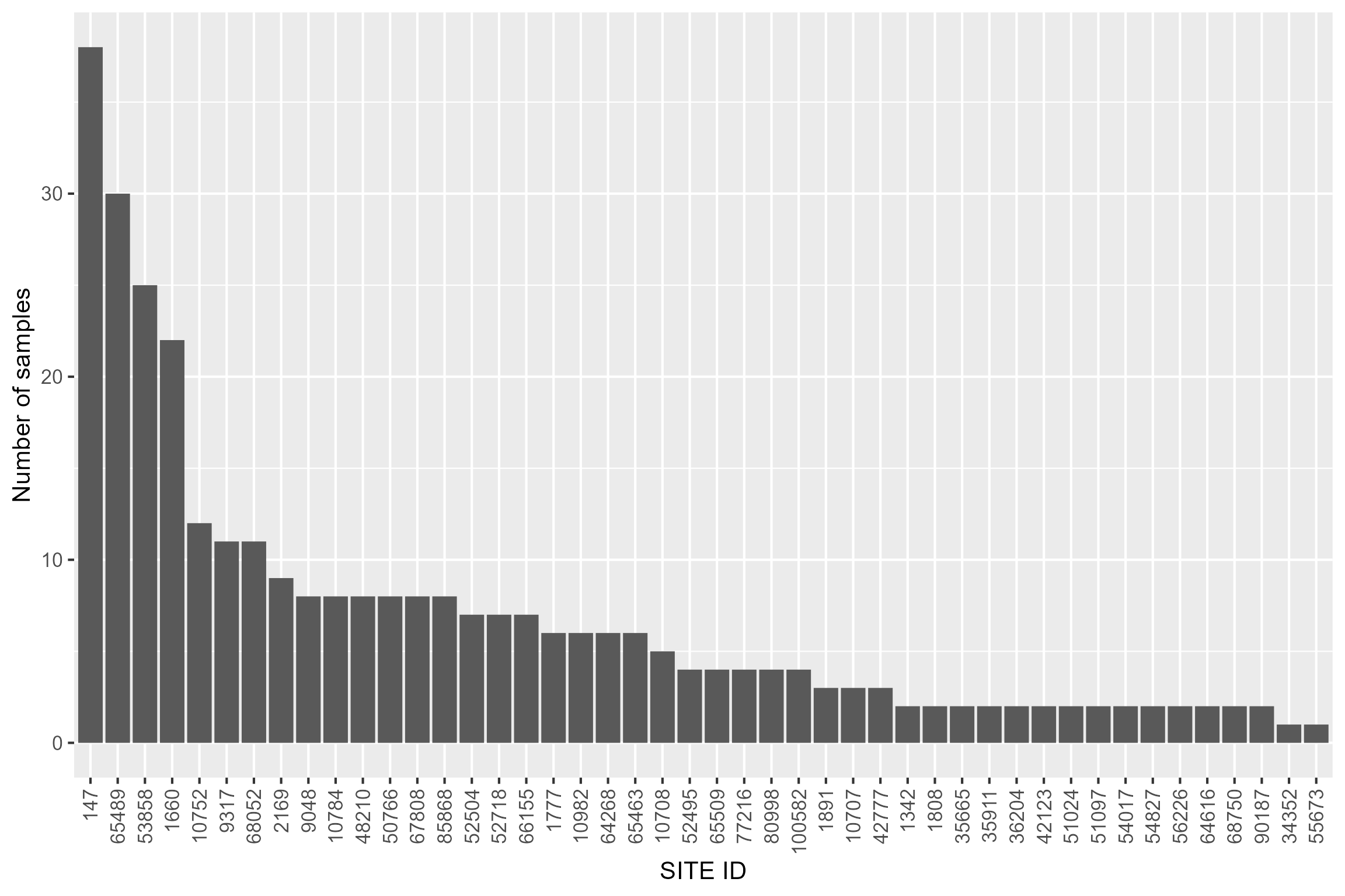
Taxonomic harmonisation
A major barrier to analysing taxonomic data is the greater formatting and processing involved. Most datasets contain ‘taxonomic redundancies’, created as taxa are identified to multiple different taxonomic levels. These need to be harmonised before the data can be analysed. Here we will look to harmonise our diatom data at species level: for diatoms, diversity within genera can be high so genus level is typically too coarse; conversely levels such as subspecies or form may be unrealistic as relatively few specimens are identified beyond species. The initial steps involved, to simplify the dataset to contain only species- and genus-level records, are as follows:
- Remove records of unidentified taxa or taxa identified to very coarse resolutions (e.g. phylum, order) that cannot realistically be assigned to a species
- Revert taxa recorded beyond species level (e.g. to subspecies, variety or form) back to their respective species
- Assign taxa recorded as a species aggregate or complex to the single species they are typically treated as
We can complete the latter two of these stages by querying the name
of each taxon to only retain the two words that make up its species
name, using the word() function of the stringr package, as
shown below.
# check ranks
unique(cs5_diat_tax$TAXON_RANK) ## [1] "Species" "Genus" "Variety"
## [4] "Unranked" "Form" "Subspecies aggregate"
## [7] "Species aggregate" "Suborder" "Generic hybrid"
## [10] "Order" "Phylum"
# the first step is to remove coarsely resolved or unidentified taxa
ranks_to_remove <- c("Phylum", "Order", "Suborder", "Unranked", "Functional group", "Generic hybrid")
cs5_diat_tax <- cs5_diat_tax %>% filter(!(TAXON_RANK %in% ranks_to_remove))
# next step is to revert subspecies records to species
# variety
cs5_diat_tax <- cs5_diat_tax %>% mutate(PREFERRED_TAXON_NAME = ifelse(TAXON_RANK == "Variety",
word(PREFERRED_TAXON_NAME, 1,2), PREFERRED_TAXON_NAME))
# form
cs5_diat_tax <- cs5_diat_tax %>% mutate(PREFERRED_TAXON_NAME = ifelse(TAXON_RANK == "Form",
word(PREFERRED_TAXON_NAME, 1,2), PREFERRED_TAXON_NAME))
# now harmonise any species aggregate records (in EDE these sometimes contain special characters
# like " in their name so we additionally need to remove these to ensure species names are consistent)
cs5_diat_tax <- cs5_diat_tax %>% mutate(PREFERRED_TAXON_NAME = ifelse(TAXON_RANK == "Species aggregate",
word(PREFERRED_TAXON_NAME, 1,2), PREFERRED_TAXON_NAME)) %>%
mutate_at("PREFERRED_TAXON_NAME", ~gsub('"', '', .))The next stage of processing includes harmonising (i) taxa recorded as a subspecies aggregate and (ii) any remaining taxa recorded with more than a single word genus or two word species name (common suffixes to remove include ‘type’ and ‘small forms’)
# check for any taxa recorded as a subspecies aggregate and revert to species
# here Gomphonema angustum/pumilum is the only one
cs5_diat_tax %>% filter(TAXON_RANK == "Subspecies aggregate") %>% distinct(PREFERRED_TAXON_NAME)## PREFERRED_TAXON_NAME
## 1 Gomphonema angustum/pumilum type
to_revert <- c("Gomphonema angustum","Gomphonema pumilum","Gomphonema angustum/pumilum type")
cs5_diat_tax <- cs5_diat_tax %>%
mutate(PREFERRED_TAXON_NAME = ifelse(TAXON_NAME %in% to_revert,
"Gomphonema angustum/pumilum", PREFERRED_TAXON_NAME))
# now check for any taxa still containing more than a standard genus or species name
# the best way to do this is to check for any names containing more than one space
cs5_diat_tax %>% filter(str_count(PREFERRED_TAXON_NAME, " ") > 1) %>% distinct(PREFERRED_TAXON_NAME)## PREFERRED_TAXON_NAME
## 1 Navicula - small forms
## 2 Achnanthidium minutissimum type
## 3 Encyonema - minutum-type
## 4 Planothidium - lanceolatum-type
## 5 Amphora pediculus type
## 6 Gomphonema intricatum type
## 7 Unidentified pennate diatoms
## 8 Navicula - cryptotenella-type
# remove these strings accordingly- pay careful attention to spaces
strings_to_remove <- list(' type', '-type',' - small forms',' -')
strings_to_remove <- paste(unlist(strings_to_remove), collapse = "|")
cs5_diat_tax <- cs5_diat_tax %>%
mutate_at("PREFERRED_TAXON_NAME", ~gsub(strings_to_remove, "", .))One more thing to look out for are genera with the suffix ‘(Other)’, whose TAXON_RANK is often incorrectly listed as ‘Species’. We need to correct this.
cs5_diat_tax <- cs5_diat_tax %>% mutate(TAXON_RANK = ifelse(str_detect(PREFERRED_TAXON_NAME, "Other"),
"Genus", TAXON_RANK))We are now ready to reassign any taxa recorded at genus to species level. We can do this using a nested process, assigning genera to the most plausible species by drawing on a progressively larger pool of reference data as needed, from (i) the sample harbouring the family, (ii) the site the sample was collected from and finally (iii) the EA area the site is located in.
This approach is broadly analogous to the ‘assign parent to the most numerous child at the site/in the study area’ method used in taxonomic harmonisation (Meredith et al., 2019), and can be used for processing other types of taxonomic data (e.g. invertebrate data). It has the benefit of preserving taxonomic resolution while eliminating taxa redundancies across the wider dataset (e.g. it avoids Achnanthidium and A. minutissimum being classified as distinct taxa in the final dataset).
# first we create a genus column
cs5_diat_tax <- cs5_diat_tax %>% mutate(TAXON_GENUS = word(PREFERRED_TAXON_NAME, 1))
# now, for each sample, calculate the proportional split of abundance among species in each genus
cs5_diat_tax <- cs5_diat_tax %>% mutate(ABUNDANCE = as.numeric(UNITS_FOUND_OR_SEQUENCE_READS))
cs5_diat_tax <- cs5_diat_tax %>% dplyr::group_by(SAMPLE_ID, TAXON_GENUS) %>%
dplyr::mutate(prop_of_genus_total =
ifelse(TAXON_RANK != "Genus", ABUNDANCE/sum(ABUNDANCE), NA)) %>%
ungroup()
# now assign genera to the most abundant species in each sample, site and area
# sample
cs5_diat_tax <- cs5_diat_tax %>% group_by(SAMPLE_ID, TAXON_GENUS) %>%
dplyr::mutate(ASSIGNED_TAXON_SAMPLE_LEVEL =
ifelse(TAXON_RANK == "Genus",
PREFERRED_TAXON_NAME[which.max(prop_of_genus_total)], NA)) %>%
ungroup()
# site
cs5_diat_tax <- cs5_diat_tax %>% group_by(SITE_ID, TAXON_GENUS) %>%
dplyr::mutate(ASSIGNED_TAXON_SITE_LEVEL =
ifelse(TAXON_RANK == "Genus",
PREFERRED_TAXON_NAME[which.max(prop_of_genus_total)], NA)) %>%
ungroup()
# area
cs5_diat_tax <- cs5_diat_tax %>% group_by(AGENCY_AREA, TAXON_GENUS) %>%
dplyr::mutate(ASSIGNED_TAXON_AREA_LEVEL =
ifelse(TAXON_RANK == "Genus",
PREFERRED_TAXON_NAME[which.max(prop_of_genus_total)], NA)) %>%
ungroup()
# we can now combine these assignations, in order of priority (sample > site > area)
cs5_diat_tax <- cs5_diat_tax %>%
mutate(ASSIGNED_TAXON =
coalesce(ASSIGNED_TAXON_SAMPLE_LEVEL,ASSIGNED_TAXON_SITE_LEVEL, ASSIGNED_TAXON_AREA_LEVEL))
# finally we can combine our assigned/inferred species records with our 'actual' species records
cs5_diat_tax <- cs5_diat_tax %>%
mutate(TAXON_NAME_FINAL = coalesce(ASSIGNED_TAXON, PREFERRED_TAXON_NAME))Our dataset of diatom taxa is now almost fully processed. The final stages are to:
- Check for any remaining genus records that we have not been able to assign to a species
- Aggregate abundances of duplicate taxa created during the harmonising of taxonomic levels
- Pivot the dataset so species abundances are in columns
- Calculate relative abundance of each species in each sample
# check for any remaining unassigned genera
cs5_diat_tax %>% filter(TAXON_RANK == "Genus" & TAXON_NAME_FINAL == PREFERRED_TAXON_NAME) %>%
select(PREFERRED_TAXON_NAME)## # A tibble: 53 × 1
## PREFERRED_TAXON_NAME
## <chr>
## 1 Kolbesia
## 2 Tryblionella
## 3 Pinnularia
## 4 Pinnularia
## 5 Synedra
## 6 Rossithidium
## 7 Achnanthes
## 8 Rossithidium
## 9 Achnanthes
## 10 Achnanthes
## # ℹ 43 more rows
# 53 records are still left at genus so we need to remove these
cs5_diat_tax <- cs5_diat_tax %>%
filter(!(TAXON_RANK == "Genus" & TAXON_NAME_FINAL == PREFERRED_TAXON_NAME))
# abundances of taxa with duplicate records for each sample now need to be aggregated
# first check for records with no abundance data
cs5_diat_tax %>% select(ABUNDANCE) %>%
dplyr::summarise_all(~sum(is.na(.)))## # A tibble: 1 × 1
## ABUNDANCE
## <int>
## 1 3
# remove these NAs
cs5_diat_tax <- cs5_diat_tax %>% filter(!is.na(ABUNDANCE))
# aggregate
cs5_diat_tax <- cs5_diat_tax %>% group_by(SAMPLE_ID, TAXON_NAME_FINAL) %>%
dplyr::summarise(ABUNDANCE= sum(ABUNDANCE)) %>%
ungroup()
# now we can pivot the data and calculate relative abundances
cs5_diat_tax_PV <- cs5_diat_tax %>%
pivot_wider(names_from = TAXON_NAME_FINAL, values_from = ABUNDANCE, values_fill = 0)
cs5_diat_RA <- cs5_diat_tax_PV
cs5_diat_RA[,-1] <- decostand(cs5_diat_RA[,-1], method="total")River Habitat Survey data
The import_rhs function allows the user to download
River Habitat Survey (RHS) data from Open Data.
# Import RHS data
cs5_rhs <- hetoolkit::import_rhs(surveys = cs5_rhssurveys)Variables can be renamed, modified and dropped from the data set if not needed.
Environmental data
Although we are working with diatom data, we can use the environmental base data for invertebrate sample sites as these contain potentially useful variables not included in the diatom environmental base data (e.g. distance from source, altitude). We can also use these data to derive a spatial estimate of fine sediment stress.
# Import environmental data from EDE
cs5_env_data <- hetoolkit::import_env(sites = cs5_diat_indices$SITE_ID)
# Check for NAs in substrate data
cs5_env_data %>% dplyr::select(BOULDERS_COBBLES, PEBBLES_GRAVEL, SAND, SILT_CLAY) %>%
dplyr::summarise_all(~sum(is.na(.)))## # A tibble: 1 × 4
## BOULDERS_COBBLES PEBBLES_GRAVEL SAND SILT_CLAY
## <int> <int> <int> <int>
## 1 0 0 0 0Land use data
If we want to include some representation of water quality in our
modelling but we don’t have sufficient suitable data we can explore
alternative approaches. One option would be to incorporate some kind of
qualitative measure, such as WFD physicochemical status classifications.
These can be imported using the cde package. Another option
is to use land use data as a broad proxy for spatial gradients in water
quality, which is the approach we will use here.
There are various publicly available GIS databases of catchment land use data but here we use the global database HydroATLAS (https://www.hydrosheds.org/hydroatlas). We import a dataset that has been pre-processed for our sites, to avoid downloading and storing large volumes of data, but the necessary processing steps are given below.
# download HydroATLAS
# riveratlas_shp_url <- "https://figshare.com/ndownloader/files/20087486"
# destfile_riveratlas <- "data/CaseStudy5/HydroATLAS/river_atlas_v10_shp.zip"
# options(timeout=9999)
# download.file(
# url = riveratlas_shp_url,
# destfile = destfile_riveratlas,
# method="auto",
# quiet = FALSE,
# mode = "wb",
# cacheOK = TRUE
#)
# unzip(destfile_riveratlas, exdir = sub(".zip", "", destfile_riveratlas))
# import the HydroBASINS shapefile (we want the max resolution available which is level 12)
# global_basins <- sf::st_read("data/CaseStudy5/HydroATLAS/BasinATLAS_v10_lev12.shp")
# crop shapefile to England
# url_request <- "https://environment.data.gov.uk/arcgis/rest/services/EA/AdminBoundEAandNEpublicFaceAreas/FeatureServer/0/query?where=seaward='No'&outFields=*&f=geojson"
# ea_areas <- st_read(url_request)
# sf_use_s2(FALSE)
# eng_basins <- st_intersection(global_basins, ea_areas)
# spatially join the land use data to our biology sites based on the HydroATLAS basin the site sits in
# cs5_env_data_sf <- osg_parse(cs5_env_data$NGR_10_FIG, coord_system = "WGS84") %>% as_tibble()
# cs5_env_data_sf <- cbind(cs5_env_data, cs5_env_data_sf) %>%
# dplyr::select(biol_site_id, lat, lon) %>%
# st_as_sf(., coords = c("lon", "lat"), crs = 4326)
# cs5_HA_data <- st_join(cs5_env_data_sf, eng_basins)
# map the basins and sites
# mapview(eng_basins, alpha.regions = 0.3, label=eng_basins$HYBAS_ID, col.regions="forestgreen") +
# mapview(cs5_env_data_sf, label=cs5_env_data_sf$biol_site_id, grid = FALSE)We now select and rename our land use variables of interest- here for simplicity we will just use the relative cover of arable farmland across the total catchment area upstream of our sites. Choice of land use variable(s) can be tailored to your dataset.
Combine data
We now need to join our taxonomic dataset of diatom species with our RHS, environmental base and land use data
# join environmental datasets
cs5_rhs <- left_join(cs5_rhs, master_file %>% select(rhs_survey_id, biol_site_id), by = "rhs_survey_id")
cs5_data_joined <- left_join(cs5_env_data %>%
select(WATER_BODY, biol_site_id, ALTITUDE, SLOPE, DIST_FROM_SOURCE,
WIDTH, DEPTH, ALKALINITY, FINE_SEDIMENT), cs5_HA_data, by = "biol_site_id")
cs5_data_joined <- left_join(cs5_data_joined, cs5_rhs, by = "biol_site_id")
# join with taxonomic data
cs5_diat_data <- cs5_diat_RA %>% left_join(cs5_diat_indices %>%
select(SITE_ID, SAMPLE_ID, SAMPLE_DATE),
by = "SAMPLE_ID") %>%
dplyr::rename(biol_site_id = SITE_ID)
cs5_diat_data$biol_site_id <- as.character(cs5_diat_data$biol_site_id)
cs5_diat_data <- cs5_diat_data %>% left_join(cs5_data_joined, by = "biol_site_id")Flow data
For this case study we use flow data that have already been processed, with flow statistics calculated over 6-monthly periods at a monthly timestep.
# load pre-processed flow data
cs5_flow_stats <- readRDS("data/CaseStudy5/cs5_flow_stats.RDS")Join hydrological and biological data
We can now link our flow data to our diatom sample data. We will join our spring diatom data to the preceding winter’s flow data and our autumn diatom data to flows over the preceding summer. As the diatom sample collection dates range from late March to late May in spring and early September to late November in autumn, the summer and winter flow periods will vary subtly among samples, hence the choice of a monthly timestep when calculating flow stats.
Below we use the join_he function with default settings
(Method = “A” and join_type = “add_flows”).
# first add month, year and season columns to biology data (specifying March as the start of spring)
cs5_diat_data <- cs5_diat_data %>% mutate(Month = month(SAMPLE_DATE))
cs5_diat_data <- cs5_diat_data %>% mutate(Year = year(SAMPLE_DATE))
cs5_diat_data <- cs5_diat_data %>%
mutate(Season = quarter(SAMPLE_DATE, with_year = FALSE, fiscal_start = 3)) %>%
mutate(Season = case_when(Season == "1" ~ "Spring",
Season == "2" ~ "Summer",
Season == "3" ~ "Autumn",
Season == "4" ~ "Winter"))
# remove any samples taken outside of spring and autumn
cs5_diat_data <- cs5_diat_data %>% filter(Season == "Spring" | Season == "Autumn")
# to ensure the `join_he` function works correctly we also need to remove any replicate samples
# collected from a site within the same year and season
# cs5_diat_data %>% group_by(biol_site_id, Year, Season) %>% dplyr::summarise(n=n()) %>% filter(n>1)
cs5_diat_data <- cs5_diat_data %>% distinct(biol_site_id, Year, Season, .keep_all = TRUE)
# check range of sample dates
# cs5_diat_data %>% filter(Season=="Spring") %>% group_by(Year) %>% dplyr::summarise(r = range(SAMPLE_DATE))
# cs5_diat_data %>% filter(Season=="Autumn") %>% group_by(Year) %>% dplyr::summarise(r = range(SAMPLE_DATE))
# join datasets
master_data <- master_file %>% filter(biol_site_id %in% cs5_diat_indices$SITE_ID)
cs5_flow_mapping <- master_data[, c("biol_site_id", "flow_site_id")]
cs5_diat_data <- cs5_diat_data %>% dplyr::rename(date = SAMPLE_DATE)
cs5_flow_stats_1 <- cs5_flow_stats[[1]]
cs5_diat_all <- join_he(biol_data = cs5_diat_data, flow_stats = cs5_flow_stats_1,
mapping = cs5_flow_mapping, lags = 0, method = "A", join_type = "add_flows")Modelling
We can now model the responses of our diatom data to flow and our other environmental variables using an approach called gradient forest (GF) analysis (Ellis et al., 2012; https://gradientforest.r-forge.r-project.org/). An extension of random forest analysis, GF is a flexible, nonlinear method for measuring patterns of species turnover along environmental gradients and detecting associated thresholds. This approach could provide useful evidence to supplement biomonitoring index- (e.g. LIFE- or WHPT-) based hydroecological models. We might choose an approach such as GF if we are working with a group of taxa (e.g. diatoms) or in an ecosystem type (e.g. temporary rivers) for which reliable flow biomonitoring indices are lacking. Such an approach could also be valuable if ecological responses to flow are relatively subtle, as GF can detect potentially important shifts in the abundance of individual species that may not show up in community-averaged biomonitoring index scores.
GF analysis constructs separate random forests for each species (/taxon) in a community to capture variation in its abundance across environmental gradients (predictors), before aggregating these responses to provide an indication of community-level change (species turnover). Within each random forest, split points along each environmental gradient are identified, with the aim of obtaining as homogeneous abundances as possible within the partitions either side of the split. Splits from those species models with a goodness-of-fit (R2) value >0 are then aggregated to estimate overall species turnover. A nested weighting approach is used, with each split weighted according to the improvement in model fit it yields, each species model contributing to community-level patterns relative to its goodness-of-fit, and the importance of each predictor calculated as an average R2 across species.
Significant features of GF analysis include its ability to model species responses across gradients with unevenly distributed data, by standardising the density of splits by the density of observations, and to subsequently detect thresholds of community change, defined as points where this standardised split density ratio is >1. The approach therefore offers an opportunity to identify where along a flow or abstraction gradient the most significant or abrupt shifts in species composition occur. GF can also be used simply to understand the importance of flow as an ecological driver relative to other pressures, such as water quality and habitat modification, for instance in order to prioritise restoration measures.
Data formatting
There are some final stages of data formatting needed for compatibility with running GF analysis. These are:
- Splitting our taxonomic and flow/environmental data into separate datasets
- Selecting which environmental variables we want to use in the modelling
- Splitting our samples by season
- Removing all infrequently occurring taxa (here <8 occurrences in a particular season), to ensure there are a sufficient number of observations for regression trees to be created. This minimum value can be adjusted (see below) but should never be <5.
# split taxonomic and environmental datasets
cs5_tax <- cs5_diat_all %>% select(SAMPLE_ID:`Fragilaria famelica`)
cs5_env <- cs5_diat_all %>% select(c(SAMPLE_ID, biol_site_id: max_doy_lag0))
# centre sampling year variable
cs5_env <- cs5_env %>% mutate(Year_centred = Year - 2012)
# select environmental variables to be used as model predictors
cs5_env <- cs5_env %>%
select(c(SAMPLE_ID, Season, Year_centred, ALTITUDE, DIST_FROM_SOURCE, ALKALINITY, FINE_SEDIMENT,
Arable_extent, HMSRBB, Q10z_lag0, Q95z_lag0))
# refine variable names
cs5_env <- cs5_env %>%
set_colnames(c("Sample_ID","Season","Year", "Altitude", "Dist_from_source", "Alkalinity",
"Fine_sediment", "Arable_extent", "Resectioning", "Q10", "Q95"))
cs5_tax <- cs5_tax %>% dplyr::rename(Sample_ID = "SAMPLE_ID")
# split dataset by season
cs5_env_files <- split(cs5_env, cs5_env$Season)
# now get matching taxonomic dataframes for spring and autumn
cs5_tax_grp <- left_join(cs5_tax, cs5_env %>% select(c(Sample_ID, Season)), by="Sample_ID") %>%
droplevels
cs5_tax_files <- split(cs5_tax_grp, cs5_tax_grp$Season)
# GF is regression-based so will struggle with any infrequently occurring taxa
# here we remove all taxa with <8 occurrences to ensure a sufficient number of observations for analysis
# we can remove the superfluous columns (sample ID and season) from the taxonomic data at the same time
# as we only want to retain the taxa columns
cs5_tax_files <- cs5_tax_files %>% lapply(., function(x) x[!(names(x) %in% c("Sample_ID", "Season"))]) %>%
lapply(., function(x) x %>% select(where(~ sum(. > 0) >=8)))
# we now have 85 diatom species for modelling of spring data and 94 for autumn
# the final step is to remove any superfluous columns from our environmental data
cs5_env_files <- cs5_env_files %>% lapply(., function(x) x[!(names(x) %in% c("Sample_ID", "Season"))])Run models
We are now ready to run our GF models. For each season we specify the relevant pair of environmental and taxonomic datasets.
In the arguments for the gradientForest() function we specify “ntree = 500” to create random forests each comprising 500 trees. We specify “corr.threshold = 0.5” to compute conditional rather than marginal permutation in order to guard against collinearity of predictors, and set the correlation threshold for this at 0.5. For information on other arguments type ?gradientForest or see https://gradientforest.r-forge.r-project.org/biodiversity-survey.pdf.
Note that the function may take a while to run if you have a large dataset. It may also return the warning message: “The response has five or fewer unique values. Are you sure you want to do regression?”, in which case we would look at increasing the threshold used to remove infrequently occurring taxa.
cs5_spr_GF <- gradientForest(data.frame(cs5_env_files$Spring, cs5_tax_files$Spring),
predictor.vars = colnames(data.frame(cs5_env_files$Spring)),
response.vars = colnames(data.frame(cs5_tax_files$Spring)),
ntree = 500, transform = NULL, maxLevel=2,
compact = FALSE, corr.threshold = 0.5)
cs5_aut_GF <- gradientForest(data.frame(cs5_env_files$Autumn, cs5_tax_files$Autumn),
predictor.vars = colnames(data.frame(cs5_env_files$Autumn)),
response.vars = colnames(data.frame(cs5_tax_files$Autumn)),
ntree = 500, transform = NULL, maxLevel=2,
compact = FALSE, corr.threshold = 0.5)Explore output
The first check of a GF model is to see how many species exhibit a positive R2, or in other words how many species are contributing to the output of each of our models. Here we can see that similar numbers of species contribute to the spring and autumn models.
cs5_spr_GF$species.pos.rsq ## [1] 45
cs5_aut_GF$species.pos.rsq## [1] 43Predictor importance
Next we can compare the overall importance of the various environmental predictors in our models. As we might expect for diatoms, alkalinity is the most important variable across both seasons, with altitude, distance from source and arable extent also relatively important. Flows over the preceding six months appear to be relatively unimportant, although the relative ranking of the two flow variables is logical, with (winter) Q10 more important in the spring data and (summer) Q95 in the autumn data.
cs5_spr_OI_plot <- ggplot(data.frame(importance(cs5_spr_GF)) %>%
rownames_to_column(., "Predictor") %>% magrittr::set_colnames(c("Predictor", "OI"))) +
geom_col(aes(x=reorder(Predictor, OI), y=OI)) + coord_flip() + ggtitle("Spring") +
labs(x="", y="") +
theme(axis.text = element_text(size = 12), axis.title = element_text(size = 12),
plot.title = element_text(size = 12))
cs5_aut_OI_plot <- ggplot(data.frame(importance(cs5_aut_GF)) %>%
rownames_to_column(., "Predictor") %>% magrittr::set_colnames(c("Predictor", "OI"))) +
geom_col(aes(x=reorder(Predictor, OI), y=OI)) + coord_flip() + ggtitle("Autumn") +
labs(x="", y="R2 weighted predictor importance") +
theme(axis.text = element_text(size = 12), axis.title = element_text(size = 12),
plot.title = element_text(size = 12))
cs5_OI_plots <- list(cs5_spr_OI_plot, cs5_aut_OI_plot)
gridExtra::grid.arrange(grobs = cs5_OI_plots)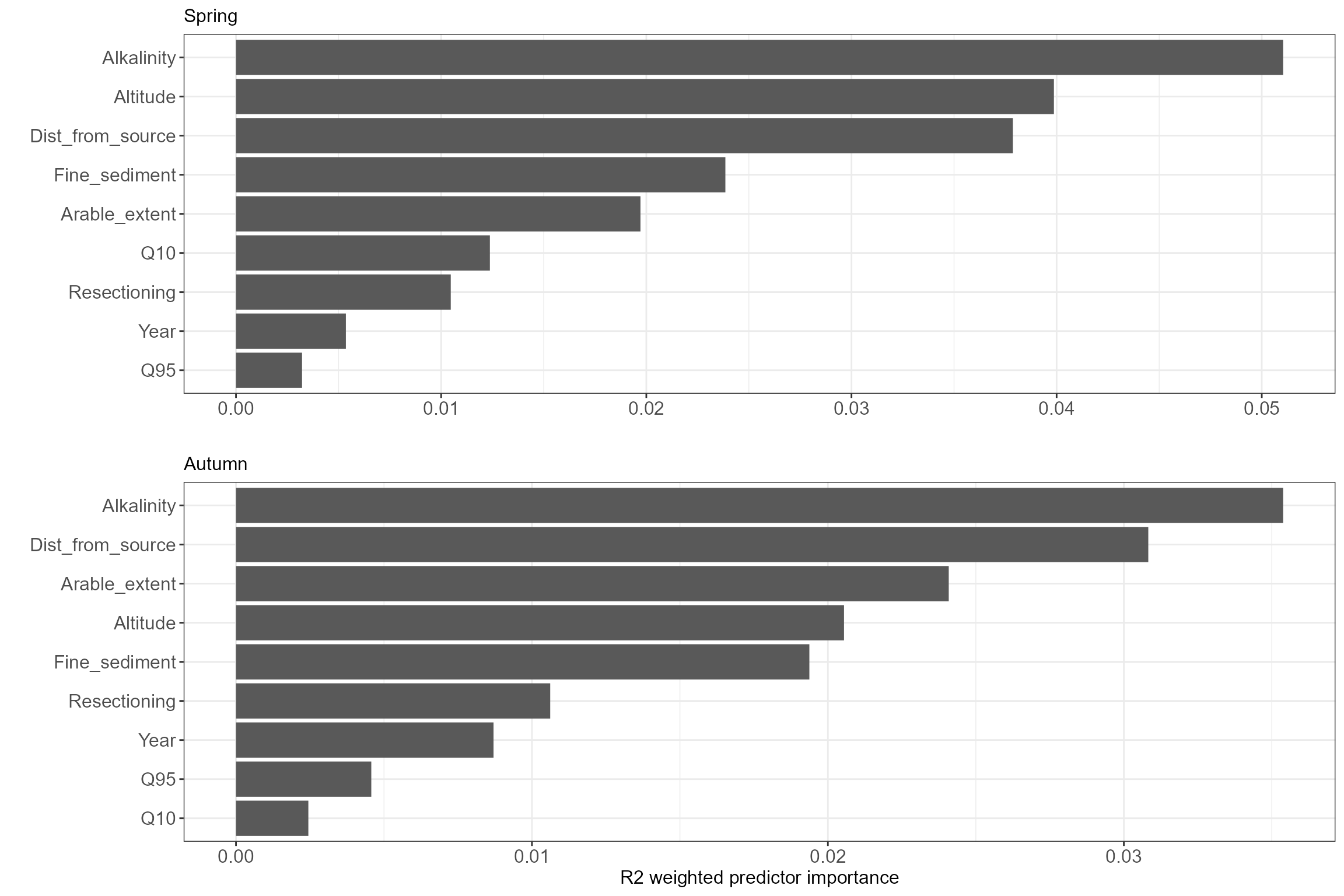
Species-level responses
We can now explore which species exhibit the highest goodness-of-fit values for the flow variables in the spring and autumn models. We select Q10 for spring and Q95 for autumn. The genus Navicula contains species that are relatively responsive to the flow gradients across both seasons, but generally the species most responsive to winter high flows appear to be different to those responsive to summer low flows.
Spring
cs5_spr_sp_tab <- cs5_spr_GF$res.u %>% mutate_at("spec", ~gsub('.', ' ', ., fixed = TRUE)) %>%
filter(var=="Q10") %>% select(c(spec, var, rsq.var)) %>%
arrange(-rsq.var) %>% head() %>% magrittr::set_colnames(c("Species", "Predictor", "R2")) %>%
mutate(across(where(is.numeric), ~ round(., digits = 3)))
cs5_spr_sp_tab %>% kable(table.attr = "style='width:60%;'") %>%
kable_minimal()| Species | Predictor | R2 |
|---|---|---|
| Navicula minima | Q10 | 0.105 |
| Staurosirella leptostauron | Q10 | 0.085 |
| Nitzschia inconspicua | Q10 | 0.083 |
| Rhoicosphenia abbreviata | Q10 | 0.075 |
| Staurosirella pinnata | Q10 | 0.057 |
| Navicula claytonii | Q10 | 0.055 |
Autumn
cs5_aut_sp_tab <- cs5_aut_GF$res.u %>% mutate_at("spec", ~gsub('.', ' ', ., fixed = TRUE)) %>%
filter(var=="Q95") %>% select(c(spec, var, rsq.var)) %>%
arrange(-rsq.var) %>% head() %>% magrittr::set_colnames(c("Species", "Predictor", "R2")) %>%
mutate(across(where(is.numeric), ~ round(., digits = 3)))
cs5_aut_sp_tab %>% kable(table.attr = "style='width:60%;'") %>%
kable_minimal()| Species | Predictor | R2 |
|---|---|---|
| Denticula tenuis | Q95 | 0.106 |
| Achnanthidium pyrenaicum | Q95 | 0.073 |
| Navicula minima | Q95 | 0.065 |
| Nitzschia inconspicua | Q95 | 0.046 |
| Staurosirella leptostauron | Q95 | 0.043 |
| Gomphonema parvulum | Q95 | 0.041 |
For these species we can now extract and plot the cumulative importance of splits in their abundance across the flow gradients. This will show us where on the flow gradients the abundance of each species is changing the most. Note that some of these particular responses may be based on relatively few occurrence records, and the main strength of GF analysis is deriving community-level trends through an aggregation of these taxon-specific responses.
The plots show that the most abrupt changes in spring abundance (steepest parts of curves) in response to winter high flows are similar across species, clustering close to a standardised Q10 value of 0. In autumn cumulative changes in abundance in response to Q95 appear to be more gradual, with the exception of Denticula tenuis. From this we might infer that in spring species responses to winter high flows exhibit signs of threshold behaviour, with sensitivity even to relatively low Q10 values, whereas in autumn sensitivity to declining low flows is similar across the gradient.
# extract cumulative importance of splits for each species
cs5_spr_cumimp <- cs5_spr_GF$res %>% dplyr::mutate_at("spec", ~gsub('.', ' ', ., fixed = TRUE)) %>%
dplyr::filter(var=="Q10", spec %in% cs5_spr_sp_tab$Species) %>% dplyr::select(spec,var,split,improve.norm) %>%
dplyr::group_by(spec) %>% arrange(split) %>% dplyr::mutate(improve.cum = cumsum(improve.norm))
cs5_aut_cumimp <- cs5_aut_GF$res %>% dplyr::mutate_at("spec", ~gsub('.', ' ', ., fixed = TRUE)) %>%
dplyr::filter(var=="Q95", spec %in% cs5_aut_sp_tab$Species) %>% dplyr::select(spec,var,split,improve.norm) %>%
dplyr::group_by(spec) %>% arrange(split) %>% dplyr::mutate(improve.cum = cumsum(improve.norm))
# create plots
cs5_spr_cumimp_plot <- ggplot(data=cs5_spr_cumimp, aes(x=split, y=improve.cum, color=spec)) +
geom_line(linewidth=1.3) + ggtitle("Spring") +
xlab("Q10") +
ylab("Cumulative importance") +
labs(color="Species") +
theme(axis.text = element_text(size = 12), axis.title = element_text(size = 12),
plot.title = element_text(size = 12), legend.text = element_text(size = 10))
cs5_aut_cumimp_plot <- ggplot(data=cs5_aut_cumimp, aes(x=split, y=improve.cum, color=spec)) +
geom_line(linewidth=1.3) + ggtitle("Autumn") +
xlab("Q95") +
ylab("Cumulative importance") +
labs(color="Species") +
theme(axis.text = element_text(size = 12), axis.title = element_text(size = 12),
plot.title = element_text(size = 12), legend.text = element_text(size = 10))
# plot
cs5_cumimp_plots <- list(cs5_spr_cumimp_plot, cs5_aut_cumimp_plot)
gridExtra::grid.arrange(grobs = cs5_cumimp_plots)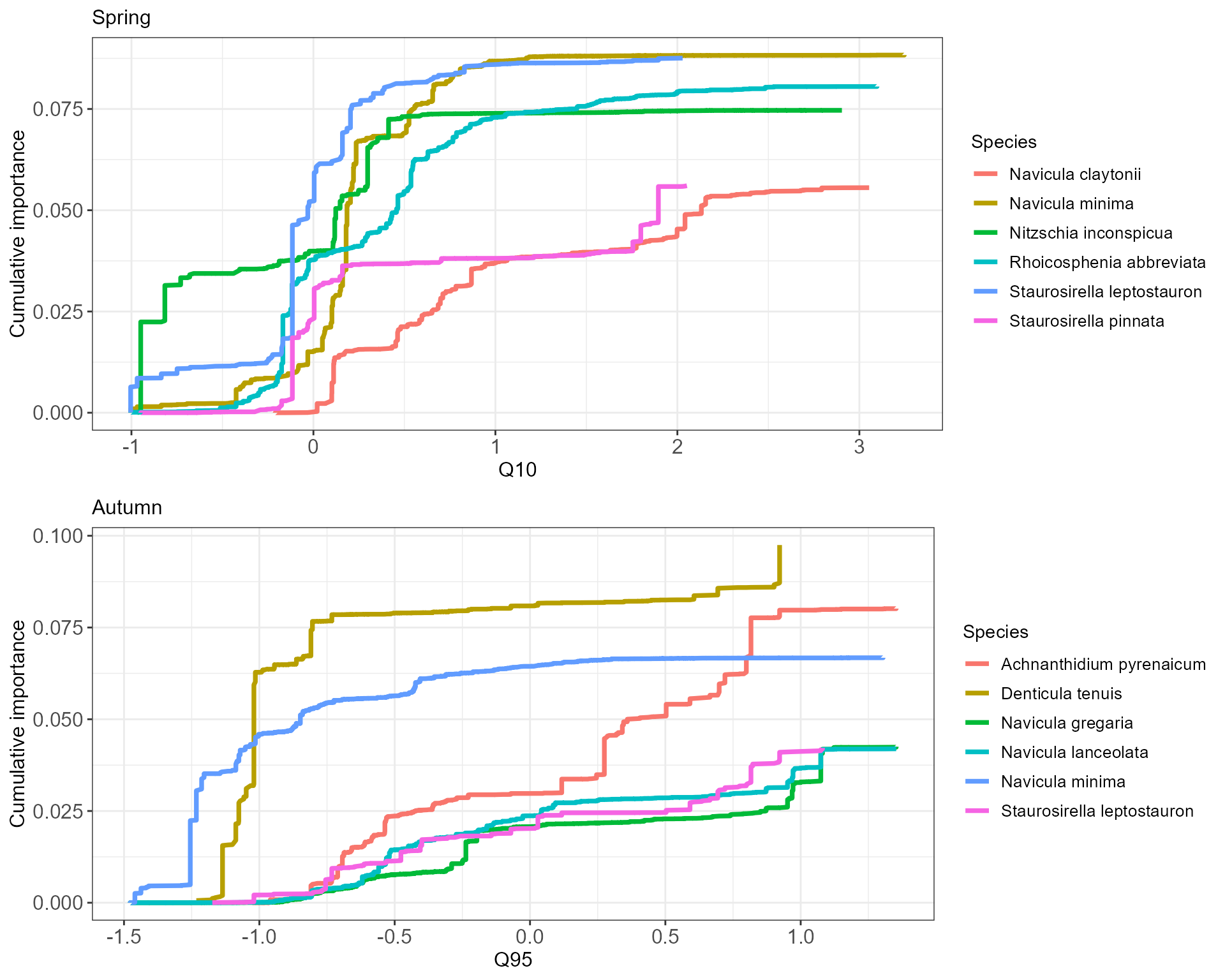
Community thresholds
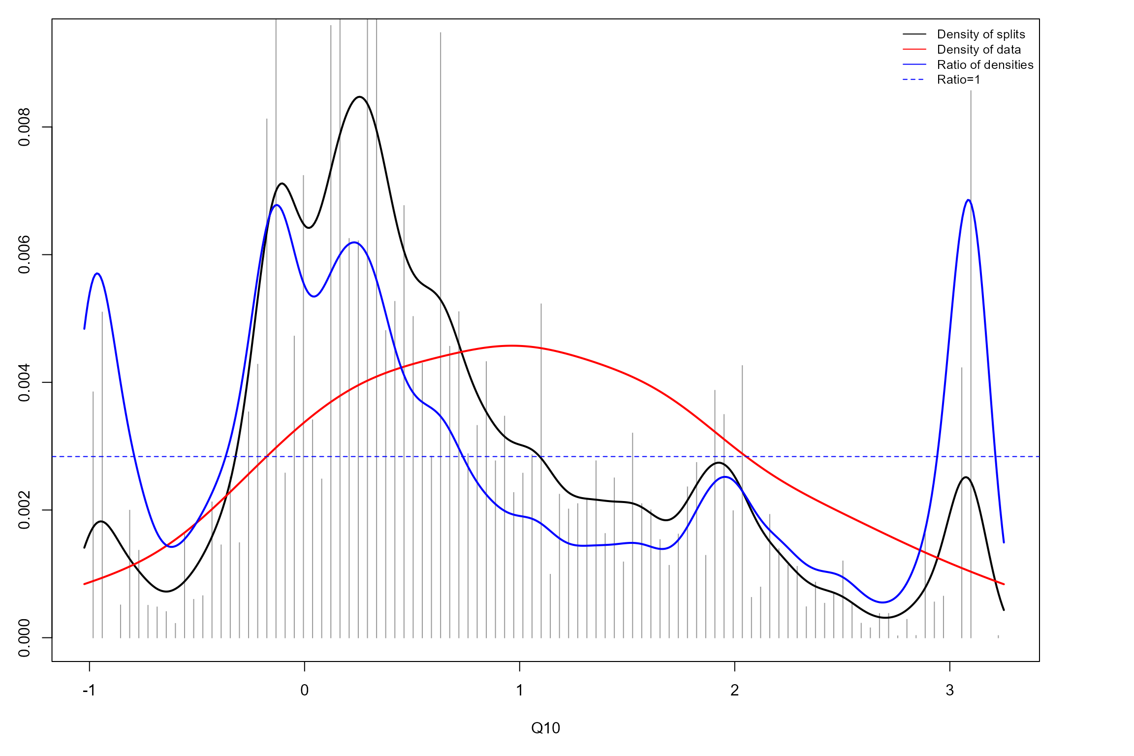
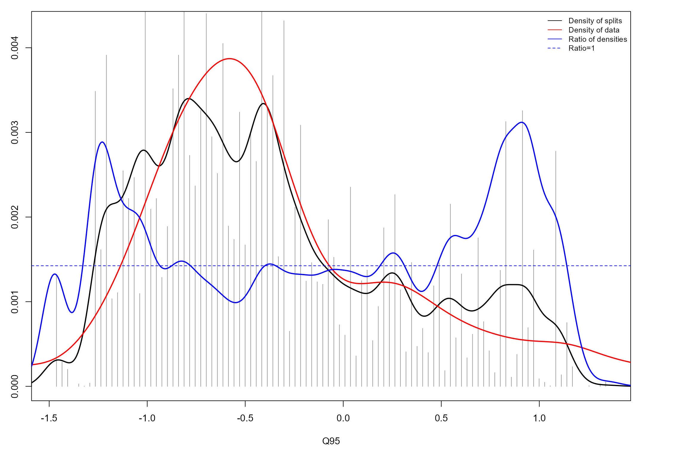
We can now produce split density plots for our GF models. These depict changes in overall community composition across the flow gradients. The solid blue lines represent the magnitude of compositional change, calculated as the density of splits at a given point on the gradient (black line) standardised by the density of observations (red line). The horizontal dotted line denotes where the ratio of split density to sample density is 1. Points where the solid blue line is greater than this ratio signify potential thresholds, where compositional change is significantly greater than at other points on the gradient.
The spring GF model identifies three thresholds, although two of these are at the tail ends of the Q10 gradient where data density is low, and so might not be reliable. This leaves a single threshold at a standardised Q10 value of approximately 0, corroborating our observations of species-specific responses above.
The autumn GF model identifies multiple thresholds across the Q95 gradient, although again several of these correspond to parts of the gradient with low data densities. The most reliable, notable threshold is apparent at a standardised Q95 value of approximately -1, again broadly consistent with the species-specific responses above. This is still not as prominent as the spring Q10 threshold detected, and variability in standardised split density across the flow gradient is generally lower in autumn than spring.
Seasonal comparison
The gradientForest package offers the option to combine
multiple GF models into a single object for purposes of comparison. Here
we combine our spring and autumn models and plot cumulative change in
abundance along both flow gradients.
# Combine GF models
cs5_comb_GF <- combinedGradientForest(Spring=cs5_spr_GF, Autumn=cs5_aut_GF)
# format data for plotting
# Q10
cs5_comb_GF_Q10 <- cbind(cs5_comb_GF$CU$Q10$Spring$x, cs5_comb_GF$CU$Q10$Spring$y,
cs5_comb_GF$CU$Q10$Autumn$y) %>% as_tibble() %>%
magrittr::set_colnames(c("Flow", "Spring", "Autumn")) %>%
pivot_longer(!Flow, names_to = "Season", values_to = "Cumulative_Importance") %>%
add_column(Predictor="Q10")
# Q95
cs5_comb_GF_Q95 <- cbind(cs5_comb_GF$CU$Q95$Spring$x, cs5_comb_GF$CU$Q95$Spring$y,
cs5_comb_GF$CU$Q95$Autumn$y) %>% as_tibble() %>%
magrittr::set_colnames(c("Flow", "Spring", "Autumn")) %>%
pivot_longer(!Flow, names_to = "Season", values_to = "Cumulative_Importance") %>%
add_column(Predictor="Q95")
# combine
cs5_season_comp <- rbind(cs5_comb_GF_Q10, cs5_comb_GF_Q95)
cs5_season_comp$Predictor <- factor(cs5_season_comp$Predictor, levels = c("Q10", "Q95"))
cs5_season_comp$Season <- factor(cs5_season_comp$Season, levels = c("Spring", "Autumn"))This comparison confirms the relative lack of significant diatom species turnover in response to summer Q10 in autumn and in response to winter Q95 in spring. We can also pick out the relatively gradual change in autumn species composition with varying summer low flows, contrasting with the much greater species turnover occurring in spring in response to winter Q10. From this we might conclude that diatom species composition is more sensitive to winter spates than summer low flow events. We should nonetheless keep in mind that that these observations are based on relatively limited data (< 120 samples from each season), with no sensitivity testing of flow windows.
# plot
cs5_season_comp %>%
ggplot(aes(Flow, Cumulative_Importance, color=Season)) + geom_line(linewidth=1.2) +
facet_grid(~Predictor) +
xlim(-2, 4) +
theme(axis.title = element_text(size=14), axis.text = element_text(size = 12),
strip.text = element_text(size=14), legend.text = element_text(size=10)) +
scale_color_manual(values=c("palegreen3", "goldenrod1"))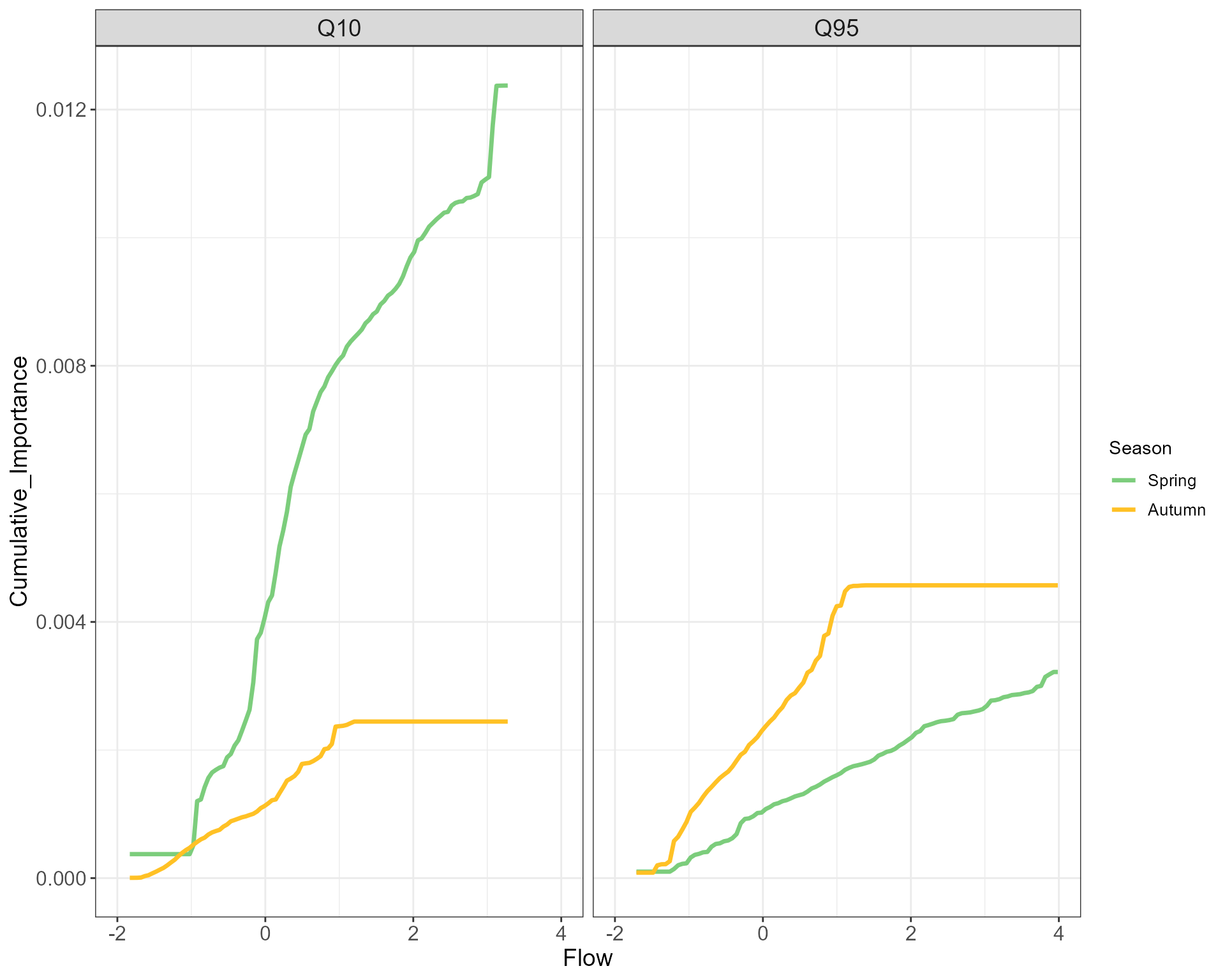
Summary
GF analysis is just one possible approach to analysing patterns of species turnover across environmental gradients, but it has the benefits of:
- being relatively sensitive to species-level shifts in abundance. It is therefore likely to offer a precautionary indication of ecological response to environmental stress
- being able to cope with samples unevenly distributed across the environmental gradient(s) of interest, which is common for gradients of abstraction pressure
- providing an intrinsic and objective means of detecting ecological thresholds
- accounting for collinearity among predictor variables by computing conditional rather than marginal importance
The same broad modelling considerations apply for GF as for biomonitoring index-based HE models, namely that sampling sites should be as free from confounding pressures as possible (and/or described by data accounting for these pressures as well as possible) and should provide maximum possible coverage of the hydrological gradient(s) of interest. GF could be used to validate the outputs of mixed models such as GLMMs and HGAMs, but is not a like-for-like substitute for these approaches as it does not explicitly incorporate random effects or interaction terms. Finally, the significance attached to any GF-derived thresholds and the taxa underlying them should be carefully considered with reference to taxa identities, the study system and the results of any accompanying analyses.
References/further reading
Chen, K. & J.D. Olden (2020). Threshold responses of riverine fish communities to land use conversion across regions of the world. Global Change Biology, 26, 4952-4965.
Ellis, N., S.J. Smith & C.R. Pitcher (2012). Gradient forests: calculating importance gradients on physical predictors. Ecology, 93, 156-168.
McKenzie, M. et al. (2024). Freshwater invertebrate responses to fine sediment stress: a multi-continent perspective. Global Change Biology, 30, e17084
Meredith, C.S., A.S. Trebitz & J.C. Hoffman (2019). Resolving taxonomic ambiguities: effects on rarity, projected richness and indices in macroinvertebrate datasets. Ecological Indicators, 98, 137-148.