Macroinvertebrates in upland rivers
APEM Ltd / Environment Agency
05 December, 2025
CaseStudy2.RmdIntroduction
This case study illustrates a typical HE Toolkit workflow using a dataset first analysed by Dunbar et al. (2010) as part of the Environment Agency-funded DRIED-UP2 study. The study used family-level macroinvertebrate LIFE scores and a mix of gauged and modelled mean daily flow data to explore how flow history and channel morphology interact to influence macroinvertebrate communities in upland rivers.
This re-analysis using the HE Toolkit has several differences from Dunbar et al. (2010) as it focuses on a reduced set of 68 macroinvertebrate sampling locations in England, uses LIFE O:E ratios rather than LIFE as the response variable, and uses updated macroinvertebrate and flow data up to 2015.
Two different modelling approaches are applied in this case study: a linear mixed-effect model, and a Generalised Additive Model (GAM). Linear models assume that the explanatory variables are linearly related to the response, whereas GAMs allow relationships between the explanatory variables and the response to be described by smooth curves or linear terms (Wood, 2017). This case study will illustrate how the same explanatory and response variables can be modeled using the two different approaches.
As this case study is intended to illustrate the application of the HE Toolkit, rather than be a comprehensive analysis in its own right, some of the analytical steps have been simplified for brevity.
This case study is optimised for viewing in Chrome.
Set-up
Install and load the HE Toolkit:
#install.packages("remotes")
library(remotes)
# Conditionally install hetoolkit from github
if ("hetoolkit" %in% installed.packages() == FALSE) {
  remotes::install_github("APEM-LTD/hetoolkit")
}
library(hetoolkit)
Install and load the other packages necessary for this case study:
if(!require(pacman)) install.packages("pacman")
pacman::p_load(knitr, DT)
pacman::p_load(lmerTest, gamm4) # for modelling
pacman::p_load(geojsonio, leaflet, rmapshaper, sf) # for maps
pacman::p_load(remotes, insight, RCurl, htmlTable, gratia, imputeTS, patchwork, ggfortify, plyr, rnrfa)

## Set ggplot theme
theme_set(theme_bw())
Metadata file
We start by importing a “metadata” file with the following columns:
- biol_site_id - a list of BIOSYS site IDs for the 68 macroinvertebrate sampling locations;
- rhs_survey_id - IDs of paired River Habitat Surveys (RHS) (note: these are survey IDs, not site IDs);
- flow_site_id - IDs of paired sites for which gauged or modelled flows are available (note that some flow sites are paired with more than one macroinvertebrate site, so there are only 56 unique flow site IDs); and
- flow_input - a vector specifying where to source the flow data for each site (gauged flows from the National River Flow Archive “NRFA” or Hydrology Data Explorer “HDE”, or modelled flows from a local “RDS” file).
# Import the metadata file containing site id's
cs2_metadata <- readxl::read_excel("data/CaseStudy2/cs2_metadata.xlsx", col_types = "text")

# Get site lists, for use with functions
cs2_rhssurvey <- cs2_metadata$rhs_survey_id
cs2_biolsites <- cs2_metadata$biol_site_id
cs2_flowsites <- cs2_metadata$flow_site_id
cs2_flowinputs <- cs2_metadata$flow_input
Look at the metadata table:
Several standardised column names are used throughout the
hetoolkit package and throughout this case study and its
associated datasets. These include:
- biol_site_id = macroinvertebrate sampling site ids.
- flow_site_id = flow gauging station ids.
-
flow = flow data, as downloaded using the
import_flowfunction - rhs_survey_id = River Habitat Survey (RHS) ids (survey id, not site id, in case multiple surveys have been undertaken at a site).
River Habitat Survey data
The import_rhs function allows the user to download
River Habitat Survey (RHS) data from Open Data.
The function either:
- downloads RHS data from Open Data, https://environment.data.gov.uk/portalstg/sharing/rest/content/items/b82d3ef3750d49f6917fff02b9341d68/data
- or imports it from a local xlsx or rds file.
Data can be optionally filtered by survey ID.
Downloaded raw data files (in .zip format) will be automatically removed from the working directory following the completed execution of the function.
Below, we use our list cs2_rhssurveys to filter the
downloaded data.
To enable the RHS data to be joined to the biology and flow data at a
later stage, it is necessary to rename the Survey ID column
to rhs_survey_id.
# Import RHS data
cs2_rhs <- hetoolkit::import_rhs(surveys = cs2_rhssurvey)
Clean RHS data
Variables can be renamed, modified and dropped from the data set if unwanted. Below we rename the variable Survey ID to rhs_survey_id to match the standardised column names used throughout the hetoolkit case studies.
# Rename survey.id to rhs_survey_id to facilitate later data joining.
cs2_rhs <- cs2_rhs %>%
  dplyr::rename(rhs_survey_id = Survey.ID, HMSRBB = Hms.Rsctned.Bnk.Bed.Sub.Score)

# use select function to keep variables of interest
cs2_rhs <- cs2_rhs %>%
  dplyr::select(rhs_survey_id, HMSRBB, HQA)

# Divide HMSRBB by 100, to avoid scaling issues in models later
cs2_rhs$HMSRBB <- cs2_rhs$HMSRBB/100
View the RHS data:
Environmental data
Import environment data
The import_env function allows the user to download
environmental base data from the Environment Agency’s Ecology and Fish
Data Explorer.
The function either:
- downloads environmental data data from https://environment.data.gov.uk/ecology-fish/downloads/INV_OPEN_DATA.zip
- or imports it from a local .csv or .rds file
Data can be optionally filtered by site ID.
When saving, the name of rds file is hard-wired to: INV_OPEN_DATA_SITES_ALL.rds.
If saving prior to filtering, the name of the filtered rds file is hard-wired to: INV_OPEN_DATA_SITE_F.rds.
Below, we use our list biolsites to filter the data from
EDE.
# Import environment data from the EDE
cs2_env_data <- hetoolkit::import_env(sites = cs2_biolsites)
Clean Environment data
# We have two sites where a value of 0 in the bed substrate composition has be read in as an NA. Lets change that to 0 to avoid NA's:
cs2_env_data[38, "SILT_CLAY"] <- 0

# We have 15 sites with no river bed composition data at all, lets remove those sites
cs2_env_data <- cs2_env_data %>%
  dplyr::filter(!is.na(PEBBLES_GRAVEL) & !is.na(SAND) & !is.na(SILT_CLAY) & !is.na(BOULDERS_COBBLES))

# Load in additional environment data for these sites
additional_env_data <- readRDS("data/CaseStudy2/additional_env_data.RDS")

# Join env data sets together:
cs2_env_data <- rbind(cs2_env_data, additional_env_data)

# Force conductivity to a numeric data type
cs2_env_data$CONDUCTIVITY <- as.numeric(cs2_env_data$CONDUCTIVITY)
View the environmental data:
Map sites
To make a map of the biology sites, we use the environmental base
data downloaded from the EDE using import_env, this gives
us the biol_site NGR’s. The NGR’s are translated to full latitude /
longitude and matched back to the env_data.
Finally we use mapview to plot the points indicating the
sample sites. The points are labelled with the biology sample site ID,
the EA area code and the catcchment.
# Convert national grid ref (NGR) to full lat / long from env_data (from import_env function)
# WGS84 is lat/long.
temp.eastnorths <- osg_parse(cs2_env_data$NGR_10_FIG, coord_system = "WGS84") %>% as_tibble()

## Match to back to env data to give details on map
cs2_env_data_map <- cbind(cs2_env_data, temp.eastnorths) %>%
  dplyr::select(AGENCY_AREA, WATER_BODY, CATCHMENT, WATERBODY_TYPE, biol_site_id, lat, lon) %>%
  dplyr::mutate(label = paste0("<b>", as.character(biol_site_id), "</b><br/>", AGENCY_AREA, "<br/>", CATCHMENT))
## Create map
leaflet() %>%
  leaflet::addTiles() %>%
  leaflet::addMarkers(lng = cs2_env_data_map$lon, lat = cs2_env_data_map$lat, popup = cs2_env_data_map$label,
            options = popupOptions(closeButton = FALSE))
Assess site similarity
Prior to building a hydro-ecological model, it is important identify any sites that could potentially be outliers because they are physically dissimilar to the others sites in the dataset.
The plot_sitepca function performs a Principal
Components Analysis (PCA) which reduces a set of site-level
environmental variables down to two uncorrelated ‘principal components’
and plots these components as a two-dimensional scatter plot. Sites that
are closer together have more similar environmental characteristics. The
proportion of the total environmental variation explained by each
component is indicated on the axis labels. The first principal component
(PC1) is plotted on the horizontal axis, as it represents the most
dominant source of variation in the dataset. The environmental gradients
represented by the two axes can be interpreted by reference to the
arrows (eigenvectors), which show the direction and strength of
correlation between the principal components and the individual
environmental variables.
hetoolkit::plot_sitepca(data = cs2_env_data,
                        vars = c("ALTITUDE", "SLOPE", "WIDTH", "DEPTH", "BOULDERS_COBBLES", "PEBBLES_GRAVEL", "SAND", "SILT_CLAY"),
                        eigenvectors = TRUE,
label_by = "biol_site_id") 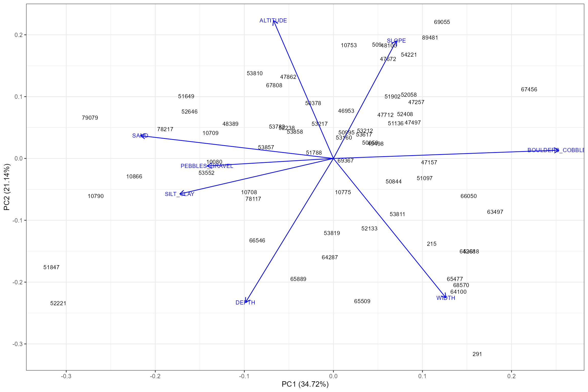
Biology data
Import data
The import_inv function imports macroinvertebrate
sampling data from the Environment Agency’s Ecology and Fish Data
Explorer. The data can either be downloaded from https://environment.data.gov.uk/ecology-fish/downloads/INV_OPEN_DATA.zip
or read in from a local .csv or .rds file. The data can be optionally
filtered by site ID and sample date.
Below, we use our list cs2_biolsites to filter the data
from the EDE. We download data for the period from 1995 (pre-1995 data
was excluded due to uncertain QA procedures in place at this time) to
2021.
# Import biology data from the EDE
cs2_biol_data <- hetoolkit::import_inv(source = "parquet", sites = cs2_biolsites, start_date = "1995-01-01", end_date = "2021-12-31")

# Set biol_site_id to character
cs2_biol_data$biol_site_id <- as.character(cs2_biol_data$biol_site_id)
Let’s view the imported data:
Calculate expected scores for macroinvertebrate indices
The predict_indices function mirrors the functionality
of the RICT2 model, by using the environmental data downloaded from the
EDE to generate expected scores under minimally impacted reference
conditions.
To run the predict_indices function, the ALTITUDE,
SLOPE, BOULDERS_COBBLES, PEBBLES_GRAVEL, SAND and SILT_CLAY fields must
all be complete:
# check for missing data
cs2_env_data %>%
  dplyr::select(ALTITUDE, SLOPE, BOULDERS_COBBLES, PEBBLES_GRAVEL, SAND, SILT_CLAY) %>%
  summarise_all(~sum(is.na(.)))
## # A tibble: 1 × 6
## ALTITUDE SLOPE BOULDERS_COBBLES PEBBLES_GRAVEL SAND SILT_CLAY
## <int> <int> <int> <int> <int> <int>
## 1 0 0 0 0 0 0Now we can calculate the expected scores using the
predict_indices function from the hetoolkit. We will
calculate all of the indices and then filter these down to the indices
we want to use for this analysis.
# Run the predict function
cs2_predict_data <- hetoolkit::predict_indices(env_data = cs2_env_data, file_format = "EDE")

# Select the columns we want to keep - for this case study we only want to keep the family-level LIFE index
cs2_predict_data <- cs2_predict_data %>%
  dplyr::select(c("biol_site_id", "SEASON", "TL3_LIFE_Fam_DistFam"))

# Rename and re-code the season column
cs2_predict_data <- cs2_predict_data %>%
  dplyr::rename(Season = SEASON) %>%
  dplyr::mutate(Season = case_when(Season == 1 ~ "Spring",
                                   Season == 2 ~ "Summer",
                                   Season == 3 ~ "Autumn",
                                   Season == 4 ~ "Winter"))

# Select the environmental variables we want to keep
cs2_env_data <- cs2_env_data %>%
  dplyr::select(biol_site_id, NGR_10_FIG, ALTITUDE, SLOPE, WIDTH, DEPTH, BOULDERS_COBBLES, PEBBLES_GRAVEL, SAND, SILT_CLAY, ALKALINITY, EASTING, NORTHING)
View the expected scores:
Join Biology and Environmental data with expected indices
Prior to joining the data, it is advisable to average results for any replicate samples collected from the same site in the same month.
Calculate O:E ratios
Now we join the observed and expected LIFE scores into a single data frame so that O:E (Observed/Expected) ratios can be calculated.
# Join predicted indices to the invertebrate data by id and season into a new data frame called cs2_biol_all
cs2_biol_all <- dplyr::left_join(cs2_biol_data, cs2_predict_data, by = c("biol_site_id", "Season"))

# Join the environmental data for later use
cs2_biol_all <-  dplyr::left_join(cs2_biol_all, cs2_env_data, by = "biol_site_id")

# Calculate LIFE O:E scores
cs2_biol_all <- cs2_biol_all %>%
  mutate(LIFE_F_E = TL3_LIFE_Fam_DistFam,
         LIFE_F_OE = LIFE_F_O / LIFE_F_E)

cs2_biol_all <- subset(cs2_biol_all, select = c(biol_site_id, Year, Season, Month, date, LIFE_F_OE))
cs2_biol_all$biol_site_id <- as.character(cs2_biol_all$biol_site_id)
Exploratory plots
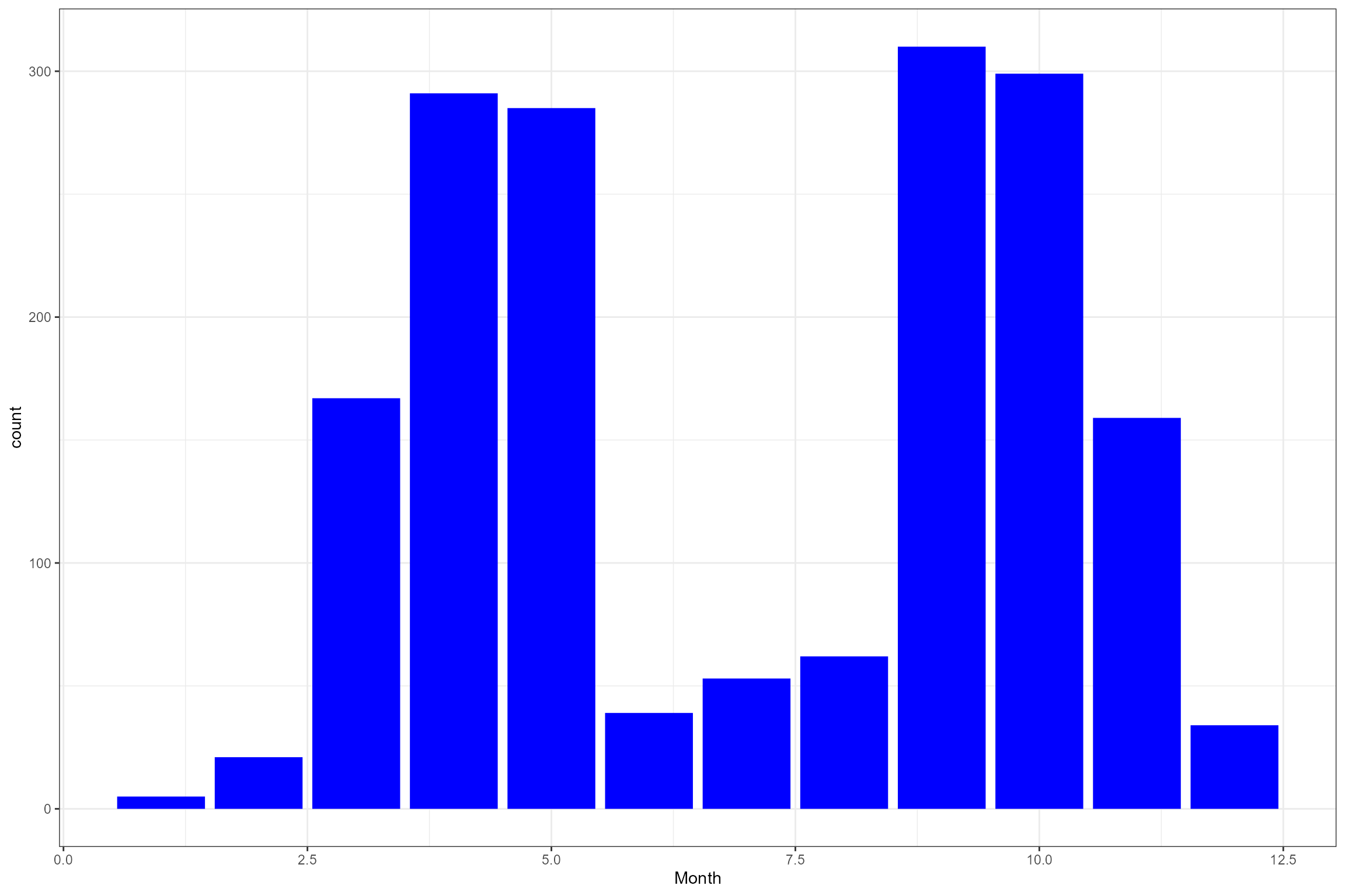
Let’s have a closer look at the biology data. The following plots show:
- The number of macroinvertebrate samples per site, by season;
- The monthly distribution of macroinvertebrate samples; and
- The distribution of the response variable (LIFE F O:E).
# Number of MI samples by site and season
ggplot(cs2_biol_all, aes(x = factor(biol_site_id, levels = rev(levels(factor(biol_site_id)))), fill = Season)) +
  geom_bar()+
  coord_flip()+
  xlab("Site") +
  ylab("Number of MI samples")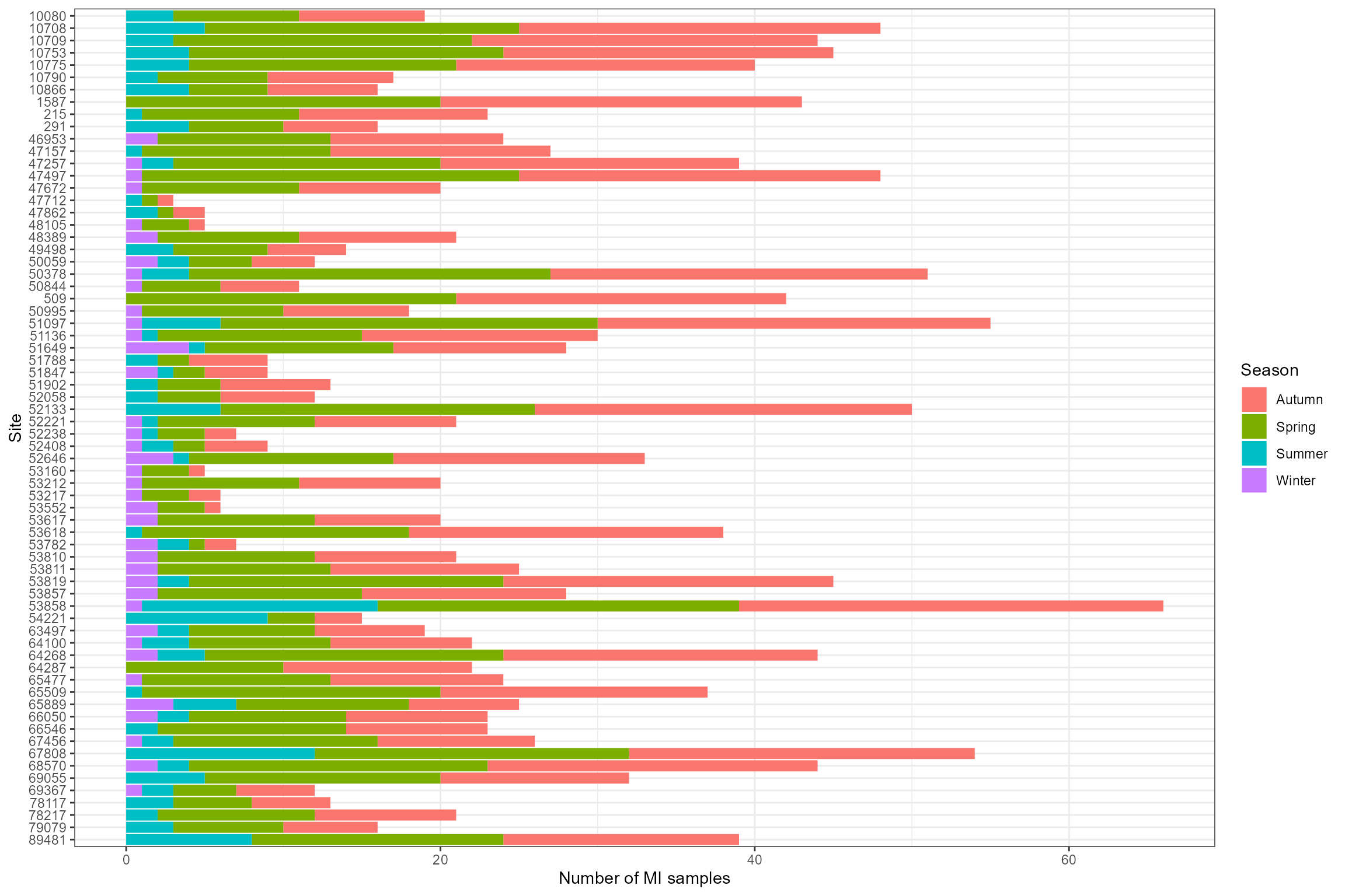
# Histogram of LIFE O:E ratios
ggplot(data = cs2_biol_all, aes(x = LIFE_F_OE)) +
  geom_histogram(color="black", fill="grey") +
xlab("LIFE F OE") 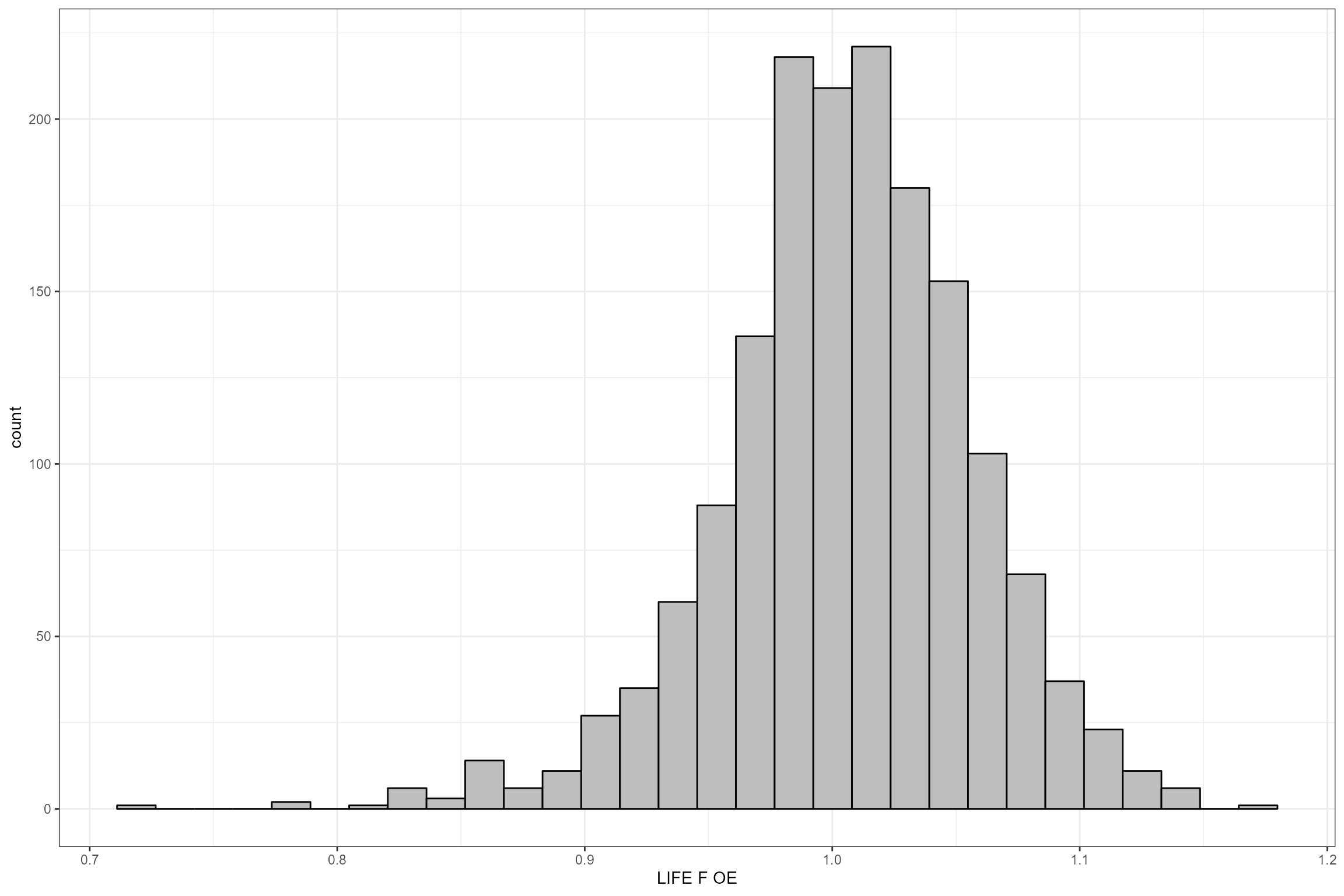
Split data by season
For this case study, the biology data needs to be split into two data frames, Spring and Autumn. The spring samples will be joined to flow statistics for the preceding six month Winter period, and the Autumn samples will be joined to flow statistics for the preceding six month Summer period.
# create cs2_spring_biol
cs2_spring_biol <- cs2_biol_all[cs2_biol_all$Season == "Spring",]

# create cs2_autumn_biol
cs2_autumn_biol <- cs2_biol_all[cs2_biol_all$Season == "Autumn",]
Flow data
Import data
import_flow is a high-level function that calls
import_nrfa, import_hde and
import_flowfiles to import data for a user-defined list of
sites.
Below, we start by importing mean daily flow data from the National River Flow Archive (NRFA) and the Hydrology Data (HDE) for a subset of 22 macroinvertebrate sites.
# Create a new data set only containing sites with flow data to import
cs2_flowinputs <- cs2_metadata[cs2_metadata$flow_input != "RDS",]

# Note that some gauging stations are paired to more than one macroinvertebrate site, so there are 16 unique gauging stations in total
unique(cs2_flowinputs$flow_site_id)

# Import flow data
cs2_flow1 <- hetoolkit::import_flow(sites = cs2_flowinputs$flow_site_id,
                                    inputs = cs2_flowinputs$flow_input,
                                    start_date = "1992-01-01", end_date = "2015-12-31")

# Remove unwanted 'input' column (so that modelled flow data can be appended - see below)
cs2_flow1 <- cs2_flow1 %>%
  dplyr::select(-input)
For the remaining sites we manually load in modelled flow data from a local RDS file:
cs2_flow2 <- readRDS("data/CaseStudy2/cs2_flow2.rds")Now we append the modelled flows to the gauged flows to give a single data frame:
# Combine cs2_flow1 and cs2_flow2 into one data frame
cs2_flow_data <- rbind(cs2_flow1, cs2_flow2)
Explore gaps in flow data
The plot_heatmap function is designed to visualise and
summarise gaps in time series data. It plots time series data for
multiple sites as a tiled heat map, and optionally produces tubular
summaries of data completeness by time period and site. Although
designed for application with flow time series data, it can be applied
to any type of numerical data, with or without a time dimension.
In the following example plot_heatmap is used to explore
gaps in the time series of mean daily flows, and then summarise how
complete the data are in each calendar month.
# Generate a heatmap of mean daily flows
cs2_heatmap <- hetoolkit::plot_heatmap(data = cs2_flow_data, x = "date", y = "flow_site_id", fill = "flow", dual = TRUE)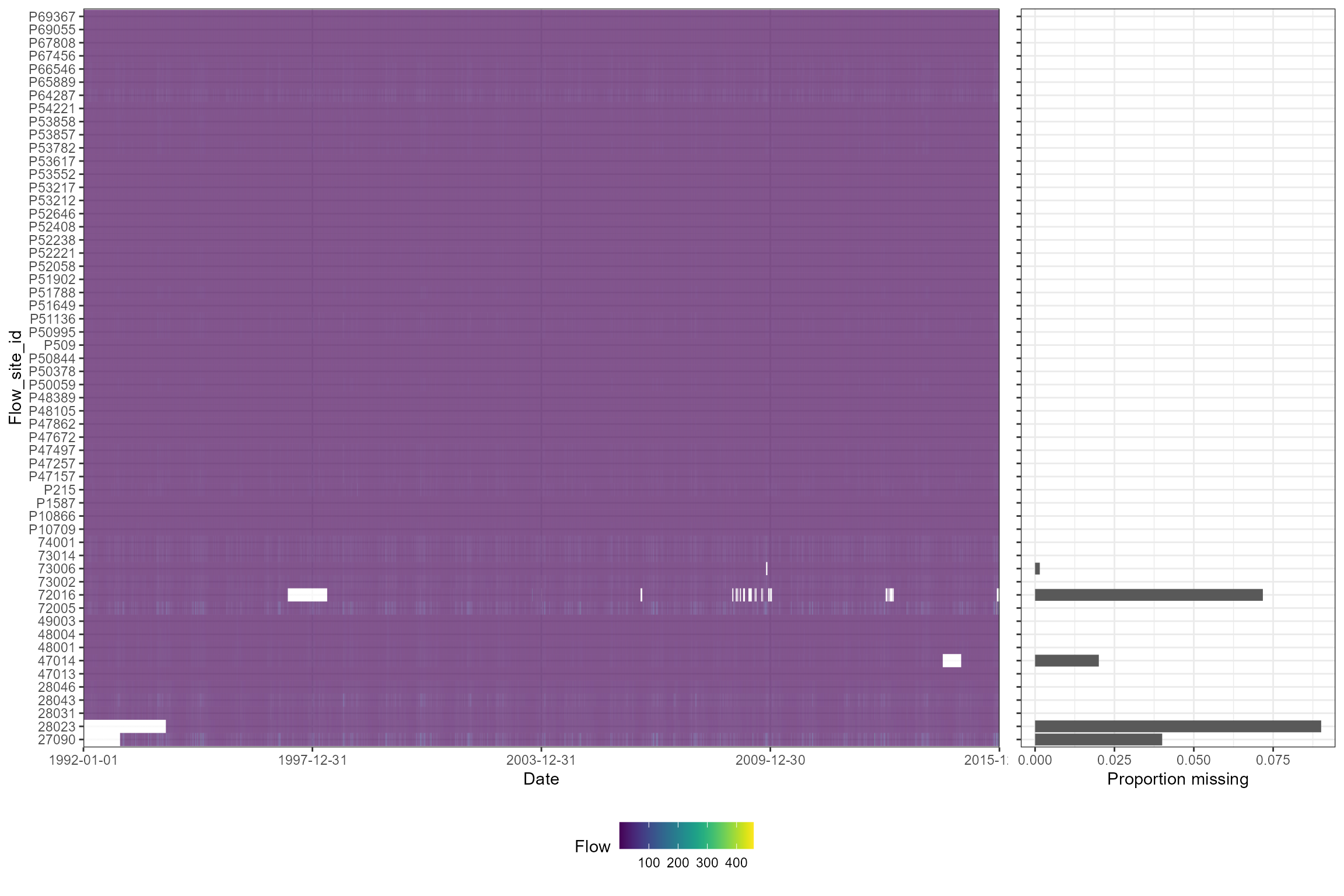
View a table of completeness statistics from each site:
Impute missing data
The impute_flow function is designed to infill missing
records in daily flow time series for one or more sites (gauging
stations) using either an interpolation or an equipercentile method.
Imputation of missing flow data can improve the later estimation of flow
statistics using the calc_flowstats function and aid
visualisation of hydro-ecological relationships using the
plot_hev function.
Here we use the equipercentile method and automatically select donor
sites to infill gaps in mean daily flow data. The donor site to be used
for each target site can be specified by the user via the
donors argument (see ?impute_flow for more detail).
# Impute flows with equipercentile method
cs2_flow_data <- hetoolkit::impute_flow(cs2_flow_data,
                                        site_col = "flow_site_id",
                                        date_col = "date",
                                        flow_col = "flow",
                                        method = "equipercentile")
Calculate flow statistics
Dunbar et al. (2010) explored the how flows in the preceding
six month period influence spring and autumn LIFE O:E ratios. Flow
statistics were calculated for winter (October-March) and summer
(April-September) periods, and these two sets of statistics were each
z-score standardised to indicate whether flows were above or below
normal for the time of year. To mirror that analysis, we run the
calc_flowstats function twice - first for winter and then
for summer - so that the winter and summer flow statistics are
standardised separately.
calc_flowstats takes a time series of measured or
modelled flows and uses a user-defined moving window to calculate a
suite of long-term and time-varying flow statistics for one or more
sites (stations).
The function uses the win_start, win_width and win_step arguments to define a moving window, which divides the flow time series into a sequence of time periods. These time periods may be contiguous, non-contiguous or overlapping.
The sequence of time periods continues up to and including the
present date, even when this extends beyond the period covered by the
input flow dataset, as this facilitates the subsequent joining of flow
statistics and ecology data by the join_he function.
It is primarily designed to work with mean daily flows (e.g. as produced by import_flow), but can also be applied to time series data on a longer (e.g. monthly) time step. Regardless, the data should be regularly spaced and the same time step should be used for all sites.
The function also requires site, date and flow data columns to be
specified in order to run. The default values for these arguments,
“flow_site_id”, “date” and “flow” respectively, match the column headers
from the outputs of the import_flow and
impute_flow functions. The defaults allow the data from
these functions to be passed without editing into
calc_flowstats, however the names can be changed as normal
to match the data supplied.
This is an updated version of the calc_flowstats
function. The first iteration of the function, which employs fixed
6-monthly spring and autumn flow periods, remains available using
calc_flowstats_old.
Note that calc_flowstats returns a list of two data
frames. The first contains a suite of time-varying flow statistics for
every time period at every site, and is extracted using [[1]]. See
?calc_flowstats for definitions of these statistics. The
second data frame contains long-term flow statistics and can be
extracted using [[2]].
# Calculate flow statistics for summer periods only
cs2_summer_flowstats <- hetoolkit::calc_flowstats(cs2_flow_data, site_col = "flow_site_id",
                                                  date_col = "date",
                                                  flow_col = "flow",
                                                  win_start = "1993-04-01",
                                                  win_width = "6 months",
                                                  win_step = "12 month")

# Extract time-varying flow statistics from calc_flowstats output
cs2_summer_flowstats1 <- cs2_summer_flowstats[[1]]

# Remove rows where flowstats are NA (post 2015-12-31)
cs2_summer_flowstats1 <- cs2_summer_flowstats1[!is.na(cs2_summer_flowstats1$Q95z),]

# Select variables we want to keep
cs2_summer_flowstats1 <- cs2_summer_flowstats1 %>%
  dplyr::select(flow_site_id, win_no, start_date, end_date, prop_missing, mean, Q10z, Q95z)

# Save a copy as a RDS file for quick importing
saveRDS(cs2_summer_flowstats1, file = "summer_flowstats1.RDS")

# Calculate flow statistics for winter period only
cs2_winter_flowstats <- hetoolkit::calc_flowstats(cs2_flow_data, site_col = "flow_site_id",
                                                  date_col = "date",
                                                  flow_col = "flow",
                                                  win_start = "1993-10-01",
                                                  win_width = "6 months",
                                                  win_step = "12 months")

# Extract time-varying flow statistics from calc_flowstats output
cs2_winter_flowstats1 <- cs2_winter_flowstats[[1]]

# Remove rows where flowstats are NA (post 2015-12-31)
cs2_winter_flowstats1 <- cs2_winter_flowstats1[!is.na(cs2_winter_flowstats1$Q95z),]

# Join_he requires unique window id's for each site, as we have ran calc_flowstats twice we add 0.5 to the winter flowstats win_no
cs2_winter_flowstats1$win_no <- cs2_winter_flowstats1$win_no + 0.5

# Select the variables we want to keep
cs2_winter_flowstats1 <- cs2_winter_flowstats1 %>%
  dplyr::select(flow_site_id, win_no, start_date, end_date, prop_missing, mean, Q10z, Q95z)

# Save a copy as a RDS file for quick importing
saveRDS(cs2_winter_flowstats1, file = "winter_flowstats1.RDS")
Join hydrological and ecological data
The join_he function links biology data with
time-varying flow statistics for one or more antecedent (lagged) time
periods (as calculated by the calc_flowstats function) to
create a combined data set for hydro-ecology modelling. The function
provides two alternative methods for linking biology samples to flow
statistics for antecedent time periods: * Method = “A” (default), lag 0
is defined for each biology sample as the most recently finished time
period; * Method = “B”, lag 0 is defined as the most recently started
flow time period.
To describe the antecedent flow conditions prior to each biology sample, the time periods are labelled relative to the date of the biology sample, with lag 0 representing either the most recently finished (method = “A”) or most recently started (method = “B”) flow time period. The time period immediately prior to the Lag 0 time period is the Lag 1 period, and the period immediately prior to that is the Lag 2 period, and so on. The function allows the user to select which antecedent (lagged) time periods the biology data are joined to, e.g. lag = c(0,1,2).
The function also includes an option to specify the “join_type”:
“add_flows” (default) produces a data set of biological metrics (response variables) and flow statistics (predictor variables) for hydro-ecological modelling.
“add_biol” produces a time series of flow statistics with associated biological metrics which can be used to assess the coverage of historical flow conditions using the
plot_rngflowsfunction.
Below we use the join_he function with method B to join the spring biology data to the most recent winter flow statistics (sw), and the autumn biology data to the most recent summer flow statistics (as). We use both “add_flows” to create a calibration dataset for hydro-ecological modelling (called HE1) and “add_biol” to create a dataset for visualisation (called HE2).
# Join Summer flow stats to Autumn biology data to using "add_flows"
cs2_as_HE1 <- hetoolkit::join_he(cs2_autumn_biol,
                                 flow_stats = cs2_summer_flowstats1,
                                 mapping = cs2_metadata,
                                 lags = 0,
                                 method = "B",
                                 join_type = "add_flows")

# Join Autumn biology data to Summer flow stats using "add_biol"
cs2_as_HE2 <- hetoolkit::join_he(cs2_autumn_biol,
                                 flow_stats = cs2_summer_flowstats1,
                                 mapping = cs2_metadata,
                                 lags = 0,
                                 method = "B",
                                 join_type = "add_biol")

# Join Winter flow stats to Spring biology data using "add_flows"
cs2_sw_HE1 <- hetoolkit::join_he(cs2_spring_biol,
                                 flow_stats = cs2_winter_flowstats1,
                                 mapping = cs2_metadata,
                                 lags = 0,
                                 method = "B",
                                 join_type = "add_flows")

# Join Spring biology data to Winter flow stats using "add_biol"
cs2_sw_HE2 <- hetoolkit::join_he(cs2_spring_biol,
                                 flow_stats = cs2_winter_flowstats1,
                                 mapping = cs2_metadata,
                                 lags = 0,
                                 method = "B",
                                 join_type = "add_biol")
And now bind the seasonal data back together, and join the RHS data to the HE1 (model calibration) dataset:
Exploratory plots
Assess coverage of historical flow conditions
A hydro-ecological model has a greater chance of revealing relationships between biology metrics and flow variables if the biology samples span a wide range of flow conditions. Good coverage of historical flow conditions by the biology sample data also means that the calibrated model is likely to be better at predicting biological responses under high and low flow scenarios.
The plot_rngflows function generates a scatterplot for
two flow variables and overlays two convex hulls: one showing the full
range of flow conditions experienced historically, and a second convex
hull showing the range of flow conditions with associated biology
samples. This visualisation helps identify to what extent the available
biology data span the full range of flow conditions experienced
historically.
In the following example, the Q95z and Q10z flow statistics have been selected as measures of low and high flows within each 6 month antecedent period. The first plot shows all of the data from all of the sites, and the second plot is faceted to show the data separately for each site individually. For the dataset as a whole, the biology samples appear to provide excellent coverage of historical flow conditions.
hetoolkit::plot_rngflows(data = cs2_HE2, flow_stats = c("Q95z_lag0","Q10z_lag0"), biol_metric = "LIFE_F_OE", wrap_by = NULL)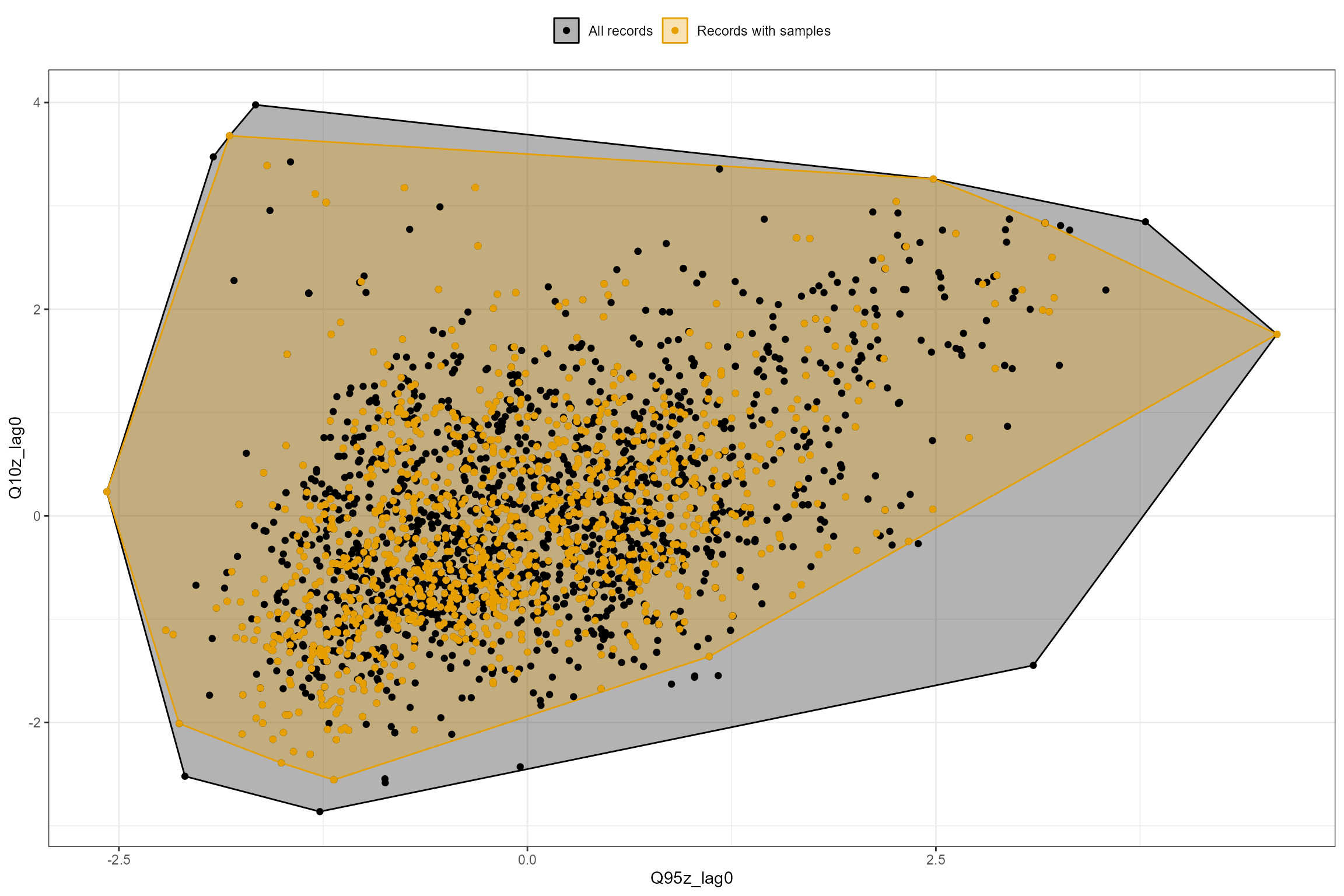
# And group by site id
hetoolkit::plot_rngflows(data = cs2_HE2, flow_stats = c("Q95z_lag0","Q10z_lag0"), biol_metric = "LIFE_F_OE", wrap_by = "biol_site_id", label = "Year")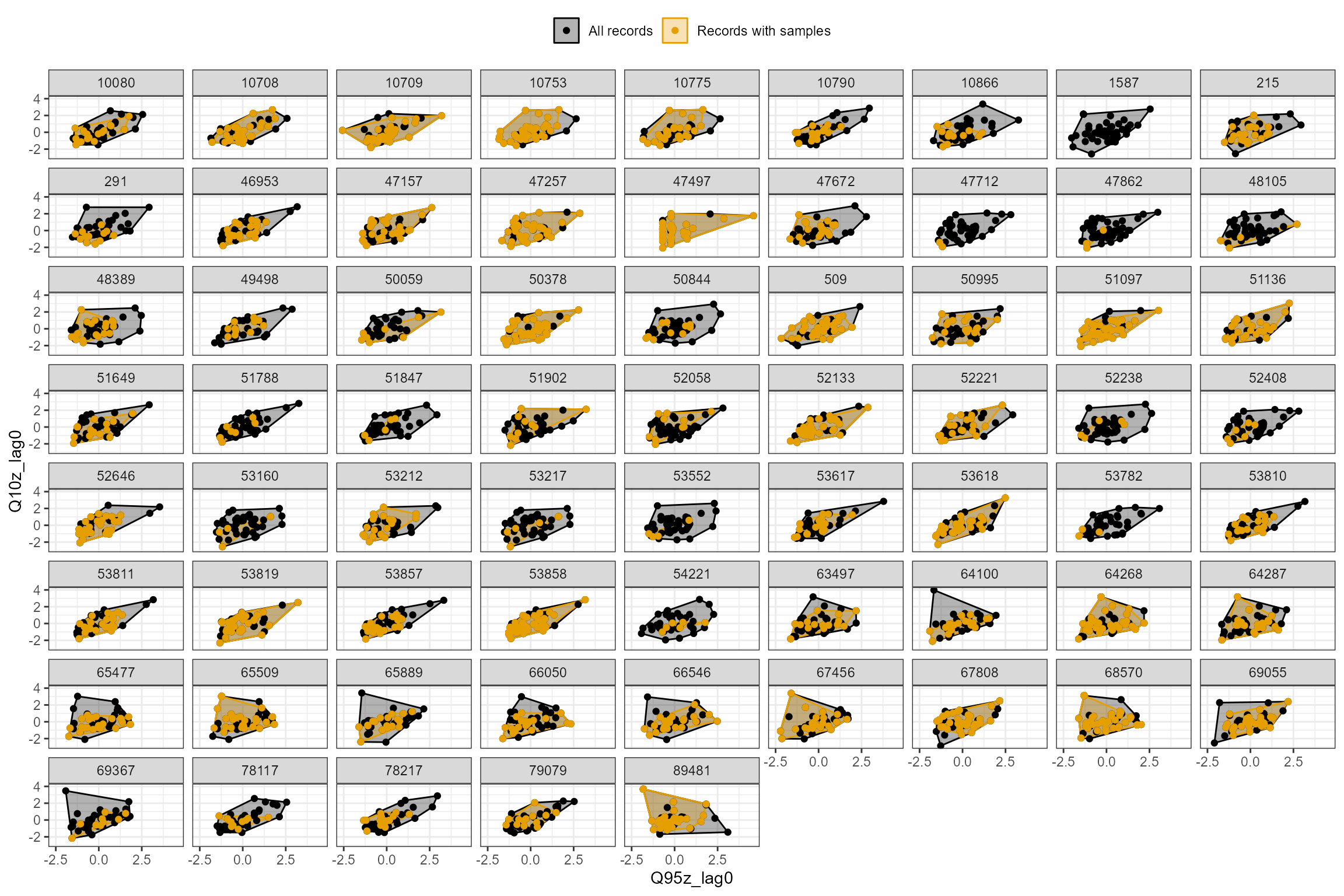
HEV plots
The plot_hev function generates, for one site of
interest, a time series plot of biology sample data and flow summary
statistics, known as as a hydroecological validation (HEV) plot. HEV
plots provide a visual assessment of trends in the historical data, and
an initial guide to possible relationships that could be explored and
quantified using a hydroecological model.
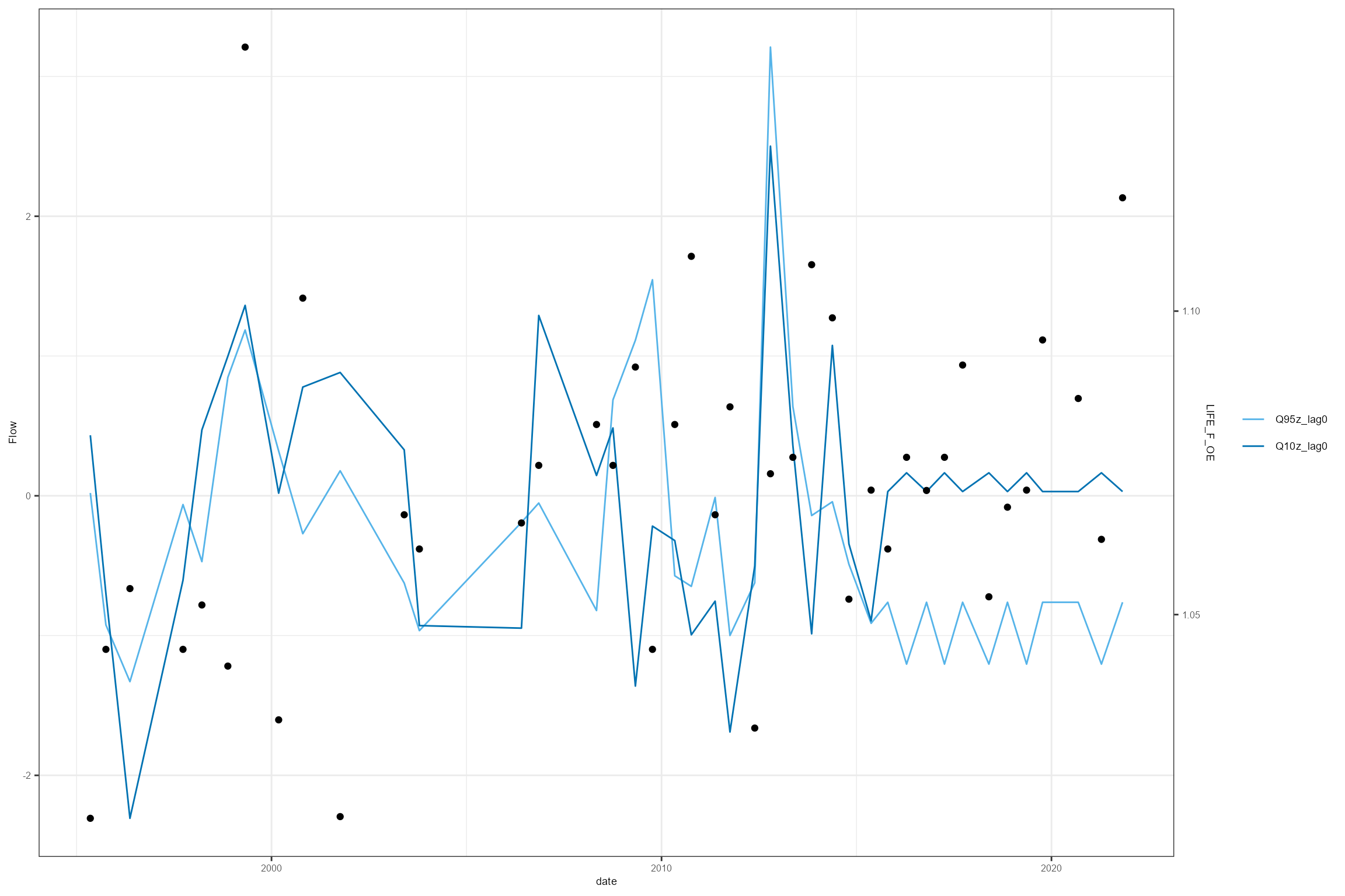
The data set created by the join_he function can be used
to produce a simple HEV plot:
cs2_HE1 %>%
  filter(biol_site_id == "53819") %>%
  dplyr::select(date, Q95z_lag0, Q10z_lag0, LIFE_F_OE) %>%
  hetoolkit::plot_hev(date_col = "date",
                      flow_stat = c("Q95z_lag0", "Q10z_lag0"),
                      biol_metric = "LIFE_F_OE")
A smarter-looking HEV plot can be created using a little manual data manipulation; this creates a “sky-scraper” plot that illustrates more clearly the time period over which the flow statistics are calculated.
# Join together summer and winter flow statistics
cs2_flowstats1 <- rbind(cs2_summer_flowstats1, cs2_winter_flowstats1)

# Create two-column table mapping biology sites to flow sites
cs2_mapping <- data.frame(cs2_metadata[,c("biol_site_id", "flow_site_id")])

# Filter biology and flow data sets to sites of interest
cs2_biol_data_hev <- dplyr::filter(cs2_biol_all, biol_site_id %in% unique(cs2_mapping$biol_site_id))
cs2_flow_data_hev <- dplyr::filter(cs2_flowstats1, flow_site_id %in% unique(cs2_mapping$flow_site_id))

# Create a complete daily time series for each biology site
cs2_hev_data <- expand.grid(
  biol_site_id = unique(cs2_biol_data_hev$biol_site_id),
  date = seq.Date(as.Date("1993-01-01"), as.Date("2015-12-31"), by = "day"),
  stringAsFactor = FALSE)

# Create Month and Year columns on which to join the 6-monthly flow statistics
cs2_hev_data <- cs2_hev_data %>%
  mutate(Month = lubridate::month(date),
         Year = lubridate::year(date))

# Join in biology data
cs2_hev_data <- cs2_hev_data %>%
  left_join(cs2_biol_data_hev, by = c("biol_site_id", "date", "Year", "Month"))

# Join in flow statistics
cs2_hev_data <- join_he(biol_data = cs2_hev_data, flow_stats = cs2_flow_data_hev, mapping = cs2_mapping, method = "A", join_type = "add_biol")
Using this new cs2_hev_data dataset, the following
example produces a HEV plot for the LIFE_F_OE response variable for one
site of interest. However, if you have multiple response variables, you
can use multiplot = TRUE to produce multiple HEV plots.
Notice the difference in this HEV plot compared to the previous one.
cs2_hev_data %>%
  filter(biol_site_id == "53819") %>%
  dplyr::select(date, Q95z_lag0, Q10z_lag0, LIFE_F_OE) %>%
  hetoolkit::plot_hev(date_col = "date",
                      flow_stat = c("Q95z_lag0", "Q10z_lag0"),
                      biol_metric = "LIFE_F_OE")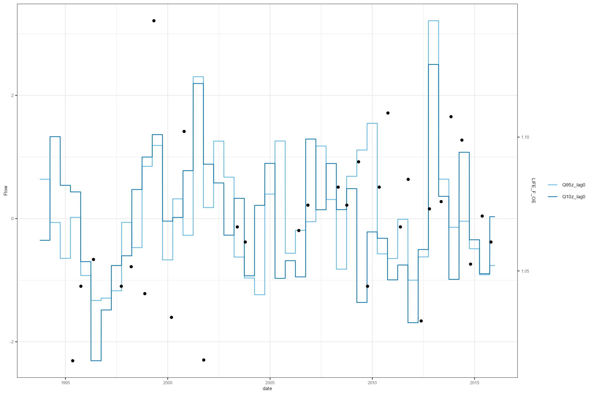

Modelling
Linear Model
Model calibration
Once the biology and flow data have been processed and assembled into
a single data frame, spatial and temporal variation in a biological
metric of interest can be modelled as a function of one or more flow
summary statistics to reveal potential hydroecological relationships.
For datasets comprising multiple sites, linear mixed-effects models
fitted using the lmer function from the lme4
package have the ability to describe a ‘global’ relationship that
applies across all sites, whilst also quantifying the degree of
variability in this relationship from site to site.
Following Dunbar et al. (2010), we model variation in LIFE
(expressed as an O:E ratio rather than as an observed score to better
control for natural variation in invertebrate community composition) as
a function of: high (Q10z_lag0) and low
(Q95z_lag0) flows in the preceding six-month winter or
summer period; Season (spring or autumn); Habitat Quality
Assessment (HQA) score, representing instream habitat
quality; Habitat Modification Score (HMSRBB) representing
the extent and severity of morphological channel alteration; and time
(Year, centered to 2005 = 0, termed Year_cen) to account
for underlying long-term trends. Selected interaction terms were also
included to explore if and how the effect of flow history varies with
season, HMSRBB and HQA (see Dunbar et al. (2010) for
details).
To reflect the hierarchical structure of the data (samples nested in sites), the models include a random intercept to account for site-to-site variation in mean LIFE O:E. Following Dunbar et al. (2010), we also include a random slope to account for site-specific time trends.
To illustrate the challenge of selecting a preferred model, we fit four competing models of varying complexity and use cross-validation to compare their predictive performance.
Candidate Models:
Model 1
# Model 1 (Model A in Table 2 of Dunbar et al. 2010)
cs2_mod1 <- lme4::lmer(LIFE_F_OE ~
                         Q10z_lag0 +
                         Season +
                         Q95z_lag0 +
                         HQA +
                         Year_cen +
                         HMSRBB +
                         Q10z_lag0:Season +
                         Q95z_lag0:HQA +
                         #Q95z_lag0:HMSRBB +
                         (Year_cen | biol_site_id),
                       data = cs2_HE1,
                       control = lmerControl(optimizer="bobyqa", optCtrl = list(maxfun = 10000)))
summary(cs2_mod1)
## Linear mixed model fit by REML ['lmerMod']
## Formula: LIFE_F_OE ~ Q10z_lag0 + Season + Q95z_lag0 + HQA + Year_cen +
## HMSRBB + Q10z_lag0:Season + Q95z_lag0:HQA + (Year_cen | biol_site_id)
## Data: cs2_HE1
## Control: lmerControl(optimizer = "bobyqa", optCtrl = list(maxfun = 10000))
##
## REML criterion at convergence: -5654.5
##
## Scaled residuals:
## Min 1Q Median 3Q Max
## -4.3600 -0.6234 -0.0211 0.6244 4.0127
##
## Random effects:
## Groups Name Variance Std.Dev. Corr
## biol_site_id (Intercept) 1.287e-03 0.035872
## Year_cen 2.640e-06 0.001625 0.18
## Residual 9.533e-04 0.030876
## Number of obs: 1467, groups: biol_site_id, 67
##
## Fixed effects:
## Estimate Std. Error t value
## (Intercept) 9.764e-01 2.996e-02 32.589
## Q10z_lag0 1.781e-03 1.259e-03 1.415
## SeasonAutumn -1.732e-03 1.631e-03 -1.062
## Q95z_lag0 1.652e-02 5.131e-03 3.220
## HQA 6.622e-04 5.444e-04 1.216
## Year_cen 1.059e-03 2.656e-04 3.988
## HMSRBB -1.472e-03 7.499e-04 -1.963
## Q10z_lag0:SeasonAutumn 1.974e-03 1.800e-03 1.096
## Q95z_lag0:HQA -2.262e-04 9.609e-05 -2.354
##
## Correlation of Fixed Effects:
## (Intr) Q10z_0 SsnAtm Q95z_0 HQA Yer_cn HMSRBB Q10_0:
## Q10z_lag0 0.013
## SeasonAutmn -0.025 -0.005
## Q95z_lag0 0.026 -0.087 -0.027
## HQA -0.984 -0.011 -0.002 -0.026
## Year_cen 0.068 -0.030 0.004 -0.020 -0.036
## HMSRBB -0.595 -0.009 0.000 -0.004 0.526 -0.018
## Q10z_lg0:SA -0.014 -0.637 0.084 -0.027 0.011 0.004 0.010
## Q95z_l0:HQA -0.025 0.054 0.017 -0.981 0.026 0.016 0.004 -0.008Model 2
# Model 2 (Model B in Table 2 of Dunbar et al. 2010)
cs2_mod2 <- lme4::lmer(LIFE_F_OE ~
Q10z_lag0 +
Season +
Q95z_lag0 +
HQA +
Year_cen +
HMSRBB +
Q10z_lag0:Season +
#Q95z_lag0:HQA +
Q95z_lag0:HMSRBB +
(Year_cen | biol_site_id),
data = cs2_HE1,
control = lmerControl(optimizer="bobyqa", optCtrl = list(maxfun = 10000)))
summary(cs2_mod2)## Linear mixed model fit by REML ['lmerMod']
## Formula: LIFE_F_OE ~ Q10z_lag0 + Season + Q95z_lag0 + HQA + Year_cen +
## HMSRBB + Q10z_lag0:Season + Q95z_lag0:HMSRBB + (Year_cen |
## biol_site_id)
## Data: cs2_HE1
## Control: lmerControl(optimizer = "bobyqa", optCtrl = list(maxfun = 10000))
##
## REML criterion at convergence: -5650.9
##
## Scaled residuals:
## Min 1Q Median 3Q Max
## -4.3801 -0.6322 -0.0234 0.6256 4.0219
##
## Random effects:
## Groups Name Variance Std.Dev. Corr
## biol_site_id (Intercept) 1.287e-03 0.035879
## Year_cen 2.712e-06 0.001647 0.17
## Residual 9.555e-04 0.030912
## Number of obs: 1467, groups: biol_site_id, 67
##
## Fixed effects:
## Estimate Std. Error t value
## (Intercept) 0.9750976 0.0300089 32.494
## Q10z_lag0 0.0019377 0.0012588 1.539
## SeasonAutumn -0.0016729 0.0016330 -1.024
## Q95z_lag0 0.0041052 0.0011280 3.639
## HQA 0.0006850 0.0005452 1.256
## Year_cen 0.0010625 0.0002683 3.960
## HMSRBB -0.0014513 0.0007513 -1.932
## Q10z_lag0:SeasonAutumn 0.0019138 0.0018027 1.062
## Q95z_lag0:HMSRBB 0.0001463 0.0001333 1.097
##
## Correlation of Fixed Effects:
## (Intr) Q10z_0 SsnAtm Q95z_0 HQA Yer_cn HMSRBB Q10_0:
## Q10z_lag0 0.015
## SeasonAutmn -0.025 -0.006
## Q95z_lag0 0.008 -0.153 -0.045
## HQA -0.984 -0.012 -0.002 -0.003
## Year_cen 0.069 -0.030 0.004 -0.005 -0.037
## HMSRBB -0.595 -0.009 0.000 -0.012 0.526 -0.019
## Q10z_lg0:SA -0.014 -0.637 0.084 -0.154 0.011 0.005 0.010
## Q95_0:HMSRB -0.005 -0.008 -0.004 -0.458 0.002 -0.033 0.021 -0.011Model 3
# Model 3 (no interactions)
cs2_mod3 <- lme4::lmer(LIFE_F_OE ~
Q10z_lag0 +
Season +
Q95z_lag0 +
HQA +
Year_cen +
HMSRBB +
#Q10z_lag0:Season +
#Q95z_lag0:HQA +
#Q95z_lag0:HMSRBB +
(Year_cen | biol_site_id),
data = cs2_HE1,
control = lmerControl(optimizer="bobyqa", optCtrl = list(maxfun = 10000)))
summary(cs2_mod3)## Linear mixed model fit by REML ['lmerMod']
## Formula: LIFE_F_OE ~ Q10z_lag0 + Season + Q95z_lag0 + HQA + Year_cen +
## HMSRBB + (Year_cen | biol_site_id)
## Data: cs2_HE1
## Control: lmerControl(optimizer = "bobyqa", optCtrl = list(maxfun = 10000))
##
## REML criterion at convergence: -5675.3
##
## Scaled residuals:
## Min 1Q Median 3Q Max
## -4.4484 -0.6338 -0.0170 0.6231 4.0266
##
## Random effects:
## Groups Name Variance Std.Dev. Corr
## biol_site_id (Intercept) 1.292e-03 0.035940
## Year_cen 2.771e-06 0.001665 0.17
## Residual 9.551e-04 0.030905
## Number of obs: 1467, groups: biol_site_id, 67
##
## Fixed effects:
## Estimate Std. Error t value
## (Intercept) 0.9756224 0.0300376 32.480
## Q10z_lag0 0.0028140 0.0009701 2.901
## SeasonAutumn -0.0018127 0.0016269 -1.114
## Q95z_lag0 0.0048625 0.0009863 4.930
## HQA 0.0006795 0.0005458 1.245
## Year_cen 0.0010733 0.0002702 3.971
## HMSRBB -0.0014763 0.0007519 -1.963
##
## Correlation of Fixed Effects:
## (Intr) Q10z_0 SsnAtm Q95z_0 HQA Yer_cn
## Q10z_lag0 0.007
## SeasonAutmn -0.024 0.062
## Q95z_lag0 0.003 -0.383 -0.038
## HQA -0.984 -0.007 -0.003 0.000
## Year_cen 0.069 -0.036 0.003 -0.022 -0.037
## HMSRBB -0.595 -0.003 -0.001 0.000 0.526 -0.018Model 4
# Model 4 (no interactions and no random slope)
cs2_mod4 <- lme4::lmer(LIFE_F_OE ~
Q10z_lag0 +
Season +
Q95z_lag0 +
HQA +
Year_cen +
HMSRBB +
#Q10z_lag0:Season +
#Q95z_lag0:HQA +
#Q95z_lag0:HMSRBB +
(1 | biol_site_id),
data = cs2_HE1,
control = lmerControl(optimizer="bobyqa", optCtrl = list(maxfun = 10000)))
summary(cs2_mod4)## Linear mixed model fit by REML ['lmerMod']
## Formula: LIFE_F_OE ~ Q10z_lag0 + Season + Q95z_lag0 + HQA + Year_cen +
## HMSRBB + (1 | biol_site_id)
## Data: cs2_HE1
## Control: lmerControl(optimizer = "bobyqa", optCtrl = list(maxfun = 10000))
##
## REML criterion at convergence: -5617.1
##
## Scaled residuals:
## Min 1Q Median 3Q Max
## -3.9218 -0.6264 -0.0226 0.6255 3.8328
##
## Random effects:
## Groups Name Variance Std.Dev.
## biol_site_id (Intercept) 0.001321 0.03635
## Residual 0.001045 0.03233
## Number of obs: 1467, groups: biol_site_id, 67
##
## Fixed effects:
## Estimate Std. Error t value
## (Intercept) 0.9807994 0.0305781 32.075
## Q10z_lag0 0.0021103 0.0009901 2.131
## SeasonAutumn -0.0019872 0.0016992 -1.169
## Q95z_lag0 0.0052460 0.0010117 5.185
## HQA 0.0005446 0.0005567 0.978
## Year_cen 0.0007905 0.0001274 6.205
## HMSRBB -0.0015364 0.0007683 -2.000
##
## Correlation of Fixed Effects:
## (Intr) Q10z_0 SsnAtm Q95z_0 HQA Yer_cn
## Q10z_lag0 0.003
## SeasonAutmn -0.025 0.060
## Q95z_lag0 0.015 -0.382 -0.036
## HQA -0.984 -0.002 -0.003 -0.010
## Year_cen 0.039 -0.045 -0.004 0.012 -0.037
## HMSRBB -0.593 0.001 0.000 -0.009 0.523 -0.005To aid model selection, the hetoolkit package includes
two functions for performing cross-validation.
model_cv performs repeated, stratified k-fold
cross-validation, which can be used to evaluate a model’s ability to
predict the response at sites in the calibration dataset. Alternatively,
model_logocv performs leave-one-group-out cross-validation,
which can be used to evaluate a model’s ability to predict the response
at sites not in the calibration dataset. Both functions can be applied
to a linear mixed-effects model (class: lmerMod) or a hierarchical
generalized additive model (class: gam) model with a single random
grouping factor. See ?model_cv and
?model_logocv for details.
model_cv and model_logocv measure the
performance of the model under different situations, and so will not
necessarily agree on which is the best model. If the priority is to be
able to predict the response at sites in the calibration dataset, then
use model_cv; if the priority is to be able to predict the
response at sites not in the calibration dataset, then use
model_logocv.
Here we use model_cv to compare the four candidate
models fitted above. Predictive performance is measured using the Root
Mean Square Error (RMSE); lower values indicate better predictions.
r is set at 10 to give stable RMSE estimates and
control is used to help prevent model convergence
issues.
my_control = lmerControl(optimizer="bobyqa", optCtrl = list(maxfun = 10000))
# Model 1
cs2_cv_mod1 <- hetoolkit::model_cv(model = cs2_mod1,
data = cs2_HE1,
group = "biol_site_id",
k = 5,
r = 10,
control = my_control)
# Model 2
cs2_cv_mod2 <- hetoolkit::model_cv(model = cs2_mod2,
data = cs2_HE1,
group = "biol_site_id",
k = 5,
r = 10,
control = my_control)
# Model 3
cs2_cv_mod3 <- hetoolkit::model_cv(model = cs2_mod3,
data = cs2_HE1,
group = "biol_site_id",
k = 5,
r = 10,
control = my_control)
# Model 4
cs2_cv_mod4 <- hetoolkit::model_cv(model = cs2_mod1,
data = cs2_HE1,
group = "biol_site_id",
k = 5,
r = 10,
control = my_control)Model 1 has the lowest RMSE, so is the preferred model.
# Let's compare the RMSE results
cs2_cv_mod1[[1]]## [1] 0.03230274
cs2_cv_mod2[[1]]## [1] 0.03236096
cs2_cv_mod3[[1]]## [1] 0.03232983
cs2_cv_mod4[[1]]## [1] 0.03230534Model interpretation
## Linear mixed model fit by REML ['lmerMod']
## Formula: LIFE_F_OE ~ Q10z_lag0 + Season + Q95z_lag0 + HQA + Year_cen +
##     HMSRBB + Q10z_lag0:Season + Q95z_lag0:HQA + (Year_cen | biol_site_id)
##    Data: cs2_HE1
## Control: lmerControl(optimizer = "bobyqa", optCtrl = list(maxfun = 10000))
##
## REML criterion at convergence: -5654.5
##
## Scaled residuals:
##     Min      1Q  Median      3Q     Max
## -4.3600 -0.6234 -0.0211  0.6244  4.0127
##
## Random effects:
##  Groups       Name        Variance  Std.Dev. Corr
##  biol_site_id (Intercept) 1.287e-03 0.035872
##               Year_cen    2.640e-06 0.001625 0.18
##  Residual                 9.533e-04 0.030876
## Number of obs: 1467, groups:  biol_site_id, 67
##
## Fixed effects:
##                          Estimate Std. Error t value
## (Intercept)             9.764e-01  2.996e-02  32.589
## Q10z_lag0               1.781e-03  1.259e-03   1.415
## SeasonAutumn           -1.732e-03  1.631e-03  -1.062
## Q95z_lag0               1.652e-02  5.131e-03   3.220
## HQA                     6.622e-04  5.444e-04   1.216
## Year_cen                1.059e-03  2.656e-04   3.988
## HMSRBB                 -1.472e-03  7.499e-04  -1.963
## Q10z_lag0:SeasonAutumn  1.974e-03  1.800e-03   1.096
## Q95z_lag0:HQA          -2.262e-04  9.609e-05  -2.354
##
## Correlation of Fixed Effects:
##             (Intr) Q10z_0 SsnAtm Q95z_0 HQA    Yer_cn HMSRBB Q10_0:
## Q10z_lag0    0.013
## SeasonAutmn -0.025 -0.005
## Q95z_lag0    0.026 -0.087 -0.027
## HQA         -0.984 -0.011 -0.002 -0.026
## Year_cen     0.068 -0.030  0.004 -0.020 -0.036
## HMSRBB      -0.595 -0.009  0.000 -0.004  0.526 -0.018
## Q10z_lg0:SA -0.014 -0.637  0.084 -0.027  0.011  0.004  0.010
## Q95z_l0:HQA -0.025 0.054 0.017 -0.981 0.026 0.016 0.004 -0.008The preferred model with the lowest RMSE (model 1) included the fixed
predictors Q10z_lag0, Q95z_lag0,
Season, HQA, Year_cen, and
HMSRBB, plus two interaction terms, while the random
effects included intercept and Year_cen varying by site. The diagnostic
plots (see below) indicate that all of these effects were approximately
linear.
On average, LIFE O:E was lower in autumn than spring, increased with habitat diversity (HQA score) and decreased with the extent of habitat modification (HMSRBB score). There was also an underlying long-term increasing trend across all sites (Year_cen) of ca 0.03. After controlling for these influences, LIFE O:E was positively associated with the Q95z flow in the preceding six-month winter or summer period and to a lesser extent with the Q10z flow. The effect of Q10z was stronger in autumn than in spring (Q10z * season interaction), and the effect of Q95z decreased with the HQA score (Q95z * HQA interaction), indicating that macroinvertebrate communities at sites with more diverse habitat were less sensitive to antecedent low flows.
The random effects estimates showed a relatively large variance in the intercept among the 68 sites, indicating a high degree of unexplained spatial variation, but only a small variance in the Year_cen effect, indicating a similar long-term trend across all sites. The random intercepts and slopes were only weakly (r = 0.16) correlated.
In spite of the use of a smaller dataset (68 vs 87 sites) and LIFE O:E ratios in preference to LIFE scores, these results are broadly consistent with those reported by Dunbar et al. (2010).
Model diagnostics
The diag_lmer function produces a variety of diagnostic
plots for a mixed-effects regression (lmer) model. Below we create model
diagnostic plots for Model 1 as it had the lowest RMSE score.
# generate diagnostic plots
cs2_diag_plots <- diag_lmer(
model = cs2_mod1,
data = cs2_HE1,
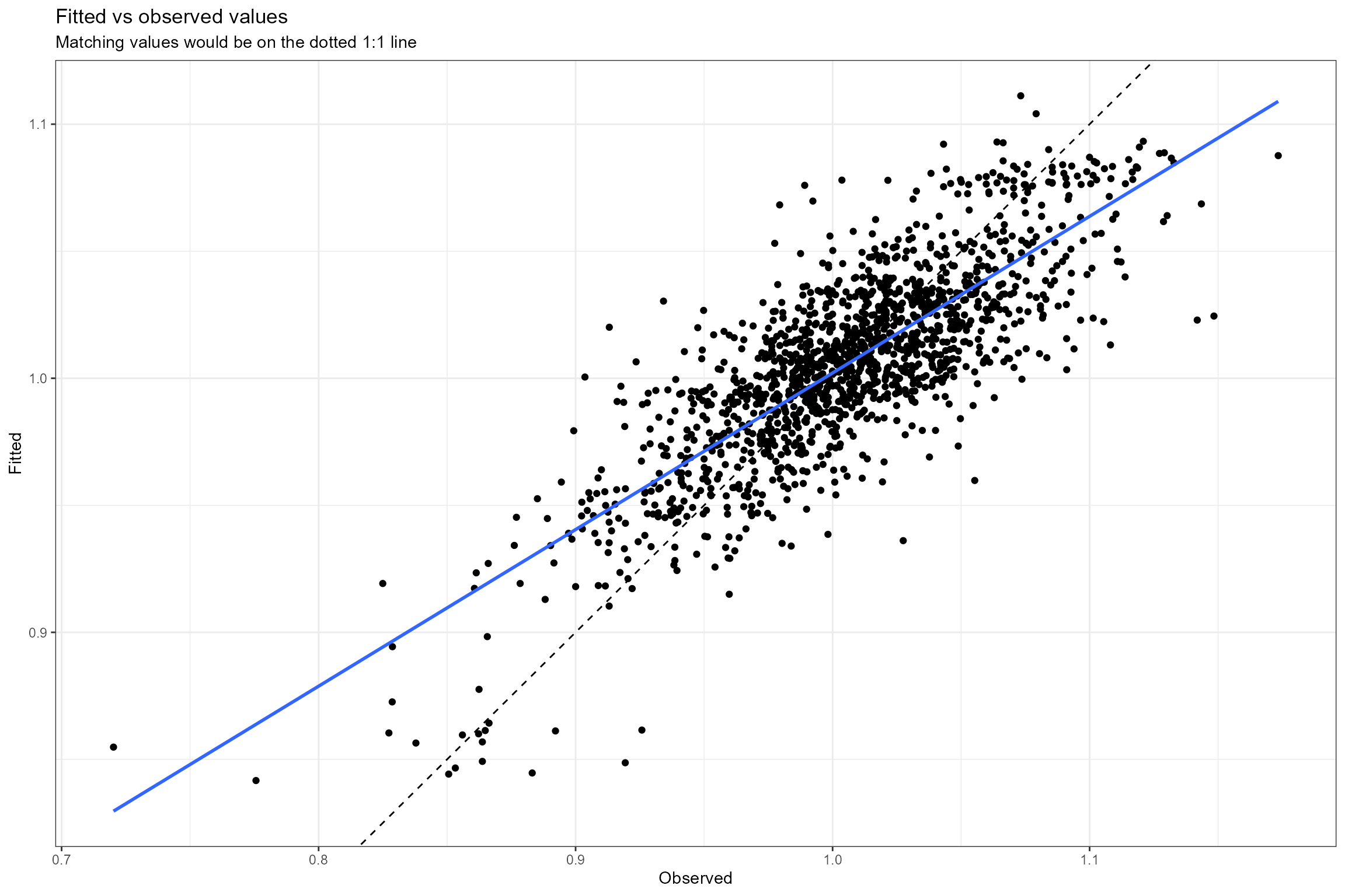
facet_by = NULL)These include:
- Fitted vs observed values. This plot shows the relationship between the fitted (predicted) and observed (true) values of the response variable. If the model fits the data well, the points should be clustered around the diagonal 1:1 line, which represents a perfect fit (fitted=observed). Here we can see the model provides a reasonably good fit to the data, but with a slight tendency to under-predict high LIFE O:E ratios and over-predict low LIFE O:E ratios (which is very common in regression modelling).
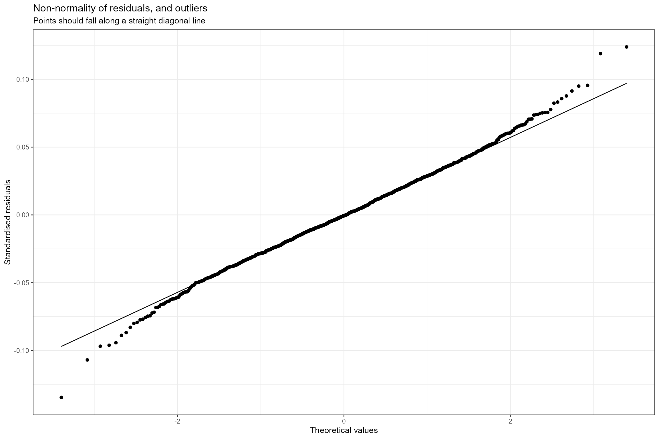
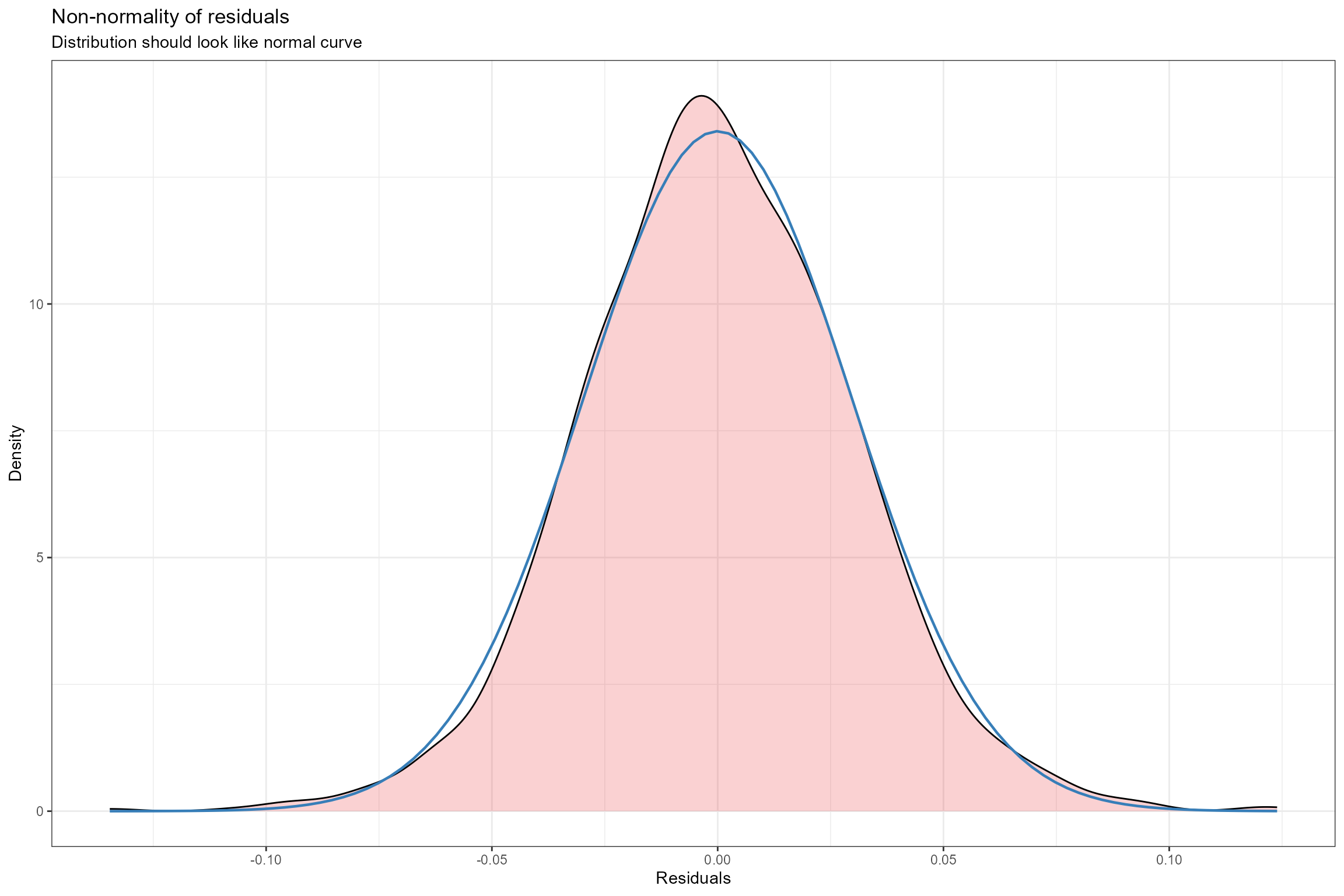
- Normal probability plot. This is a graphical technique for verifying the assumption of a normally distributed error structure. The model residuals are plotted against a theoretical normal distribution in such a way that the points should form an approximate straight line. Here we can see that the residuals conform very closely to a normal distribution, with only small deviations at the extremities.
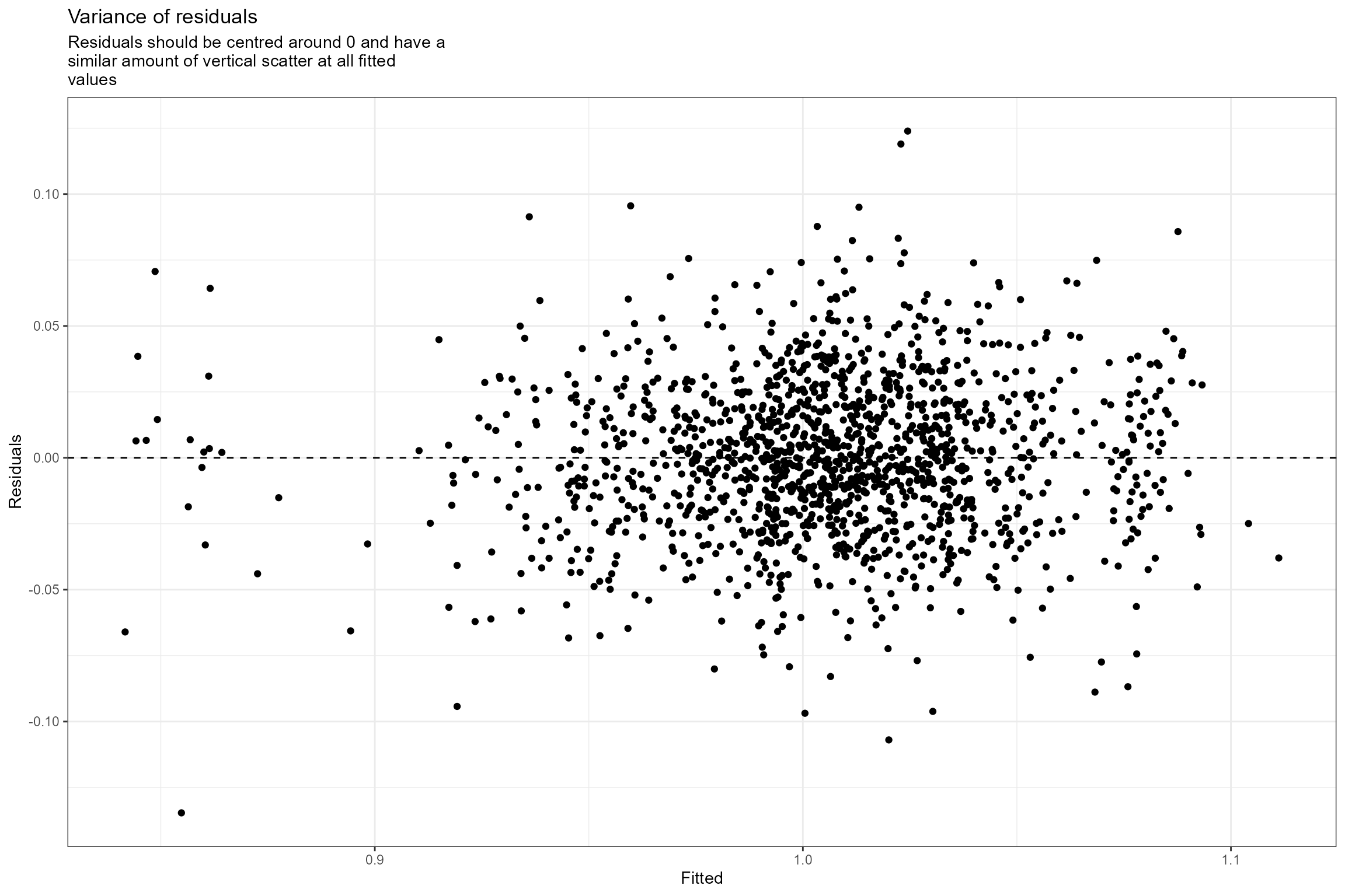
- Residuals vs fitted. This plot checks the assumption of homogeneous variances, which states that the error variance should be constant regardless of what value the response takes. Here we can see that the residuals have a similar amount of vertical scatter at all fitted values of the response, so this assumption is verified.
- Histogram of residuals. This is an alternative to plot 2 for verifying the assumption of normally distributed errors. Here we can see that the probability distribution of the model residuals (shown in pink) is very similar to a perfect normal distribution.
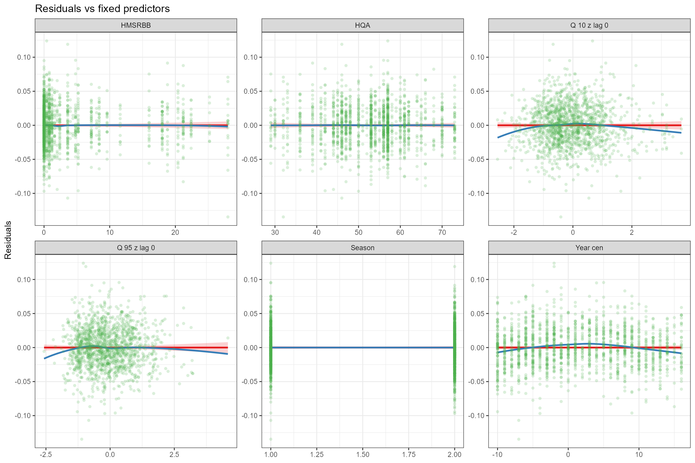
- Residuals vs model fixed predictors. To verify the assumption of linearity, the model’s residuals are plotted against each of the fixed predictors in turn. If the relationship between the response and each predictor is truly linear, then there should be no trend in the residuals. Here we can see that the linear (red) line fitted to the residuals is horizontal, indicating that the strength of the linear effects has not been over-or under-estimated. Also in most cases the loess-smoothed (blue) line is close to horizontal; there is a small departure from linearity for Q95z_lag0, Q10z_lag0 and Year_cen, but for Q95z_lag0 and Q10z_lag0 this is due to a small number of unusually low/high data points and in all cases the deviations are small, so in this example a linear model appears to provide a reasonable representation of these relationships.
Other useful diagnostic plots for lmer models
include:
- Caterpillar plots, which plot the random intercepts and slopes for each site as deviations from the global intercept and slope. Sites coloured blue are those where, all else being equal, the intercept or slope is higher than average, and red sites have lower-than-average intercepts and slopes. This confirms that there is reasonably large (+/- 0.1) variation in LIFE O:E ratios from site to site that cannot be explained by the other, fixed effects in the model. The random variance for Year_cen is much smaller, but this still translates into important differences in time trends among sites (see below for a clearer visualisation).
sjPlot::plot_model(model = cs2_mod1,
                   type = "re",
                   facet.grid = FALSE,
                   free.scale = FALSE,
                   title = NULL,
                   vline.color = "darkgrey") +
  ylim(-0.15,0.15)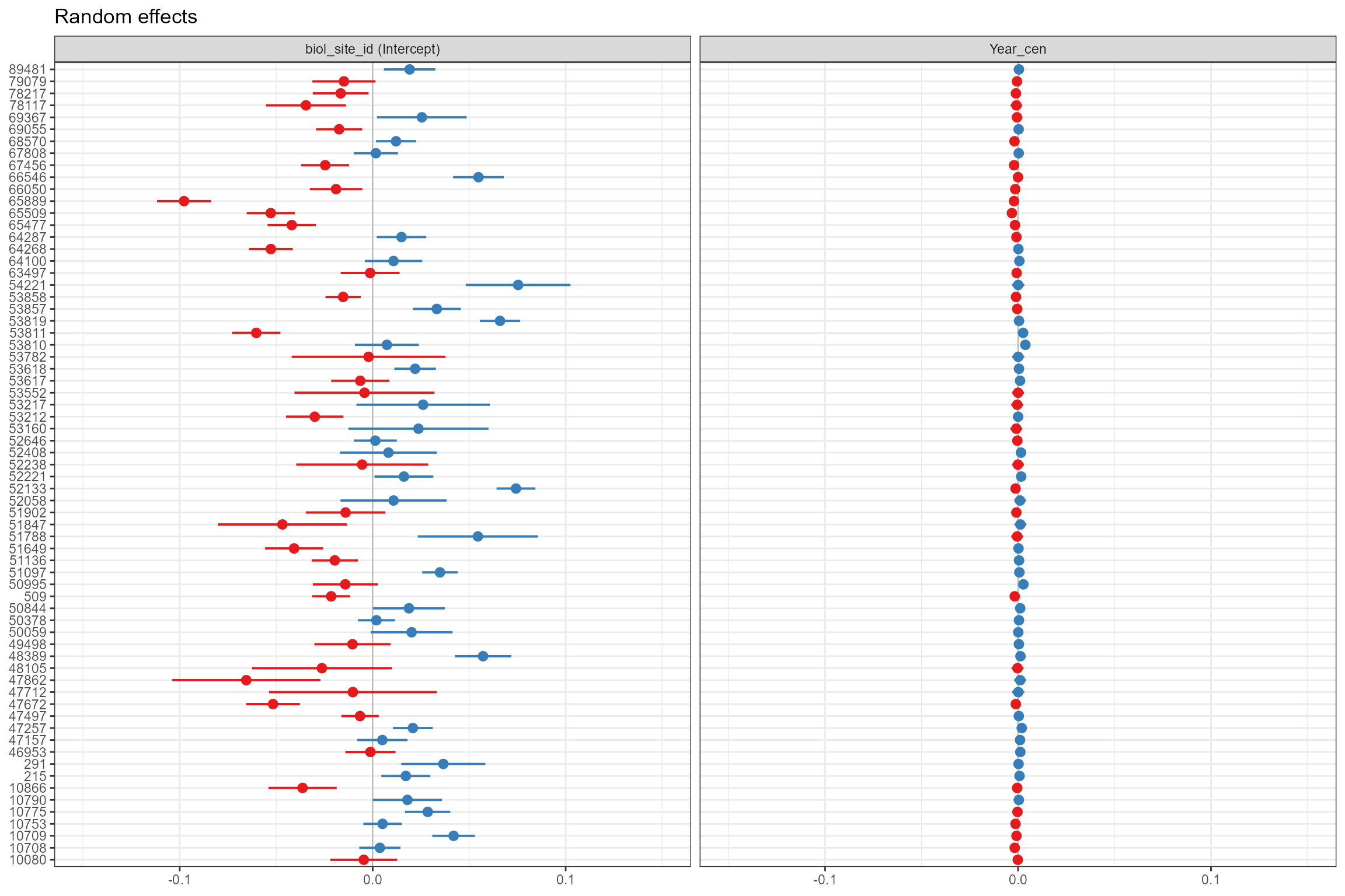
- Partial effects plots, for visualising the fixed effects that are common to all sites; these show the modelled effect of each predictor in turn when other continuous predictors are held constant at their mean values and factors are fixed at their reference level (i.e. spring for Season). This confirms the positive associations with low flows (Q95z) and habitat quality (HQA) and the negative effect of bed and bank resectioning (HMSRBB).
sjPlot::plot_model(model = cs2_mod1,
                   type = "pred",
                   pred.type = "fe",
                   title = NULL, terms= "Q95z_lag0")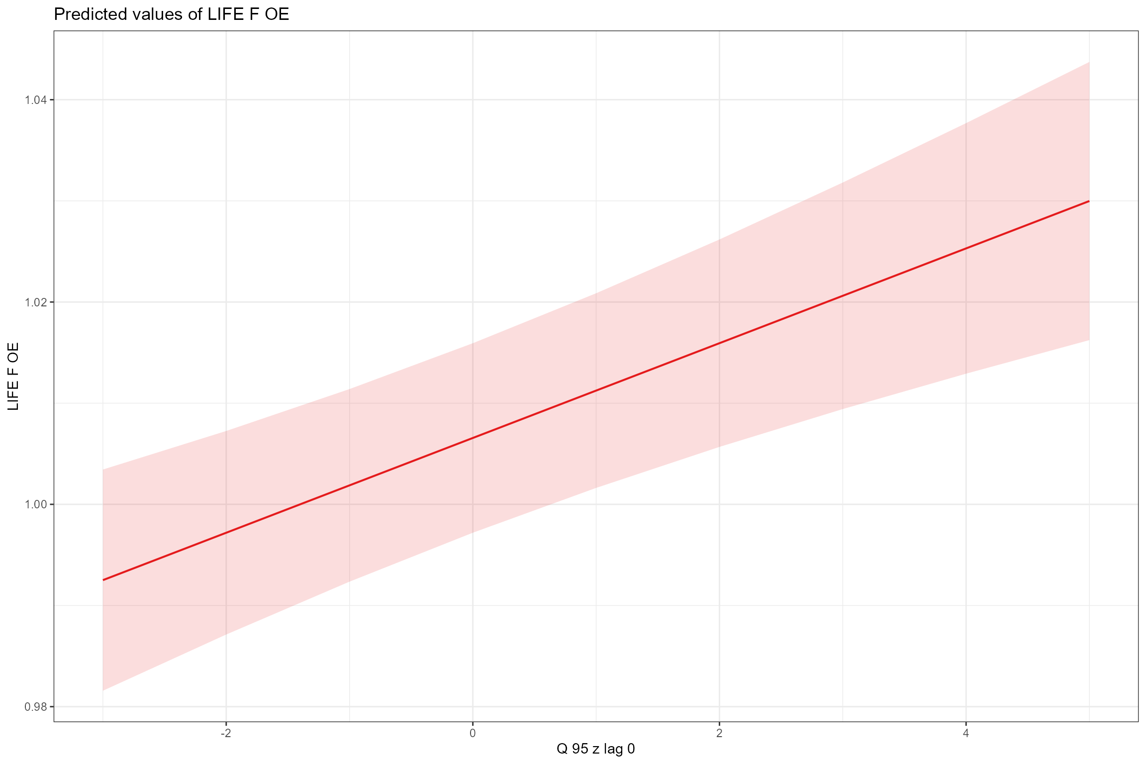
sjPlot::plot_model(model = cs2_mod1,
                   type = "pred",
                   pred.type = "fe",
                   title = NULL, terms= "HQA")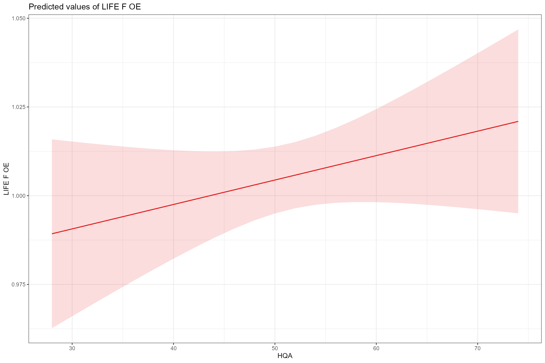
sjPlot::plot_model(model = cs2_mod1,
                   type = "pred",
                   pred.type = "fe",
                   title = NULL, terms= "HMSRBB")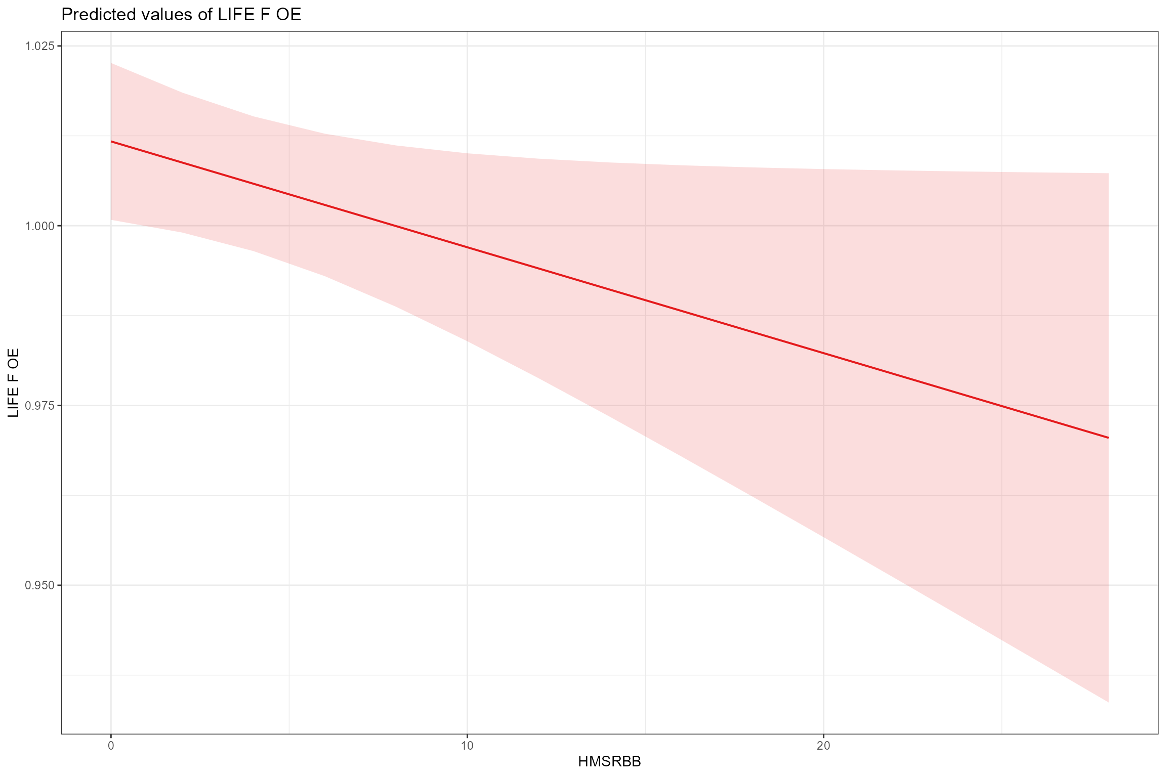
- Interaction plots, showing how the effect of one predictor depends upon the value of another predictor. Here we can see that the effect of high flows (Q10z_lag0) is marginally stronger in autumn than in spring, and that sites with poorer habitat quality (low HQA scores) are more sensitive to low flows (Q95z_lag0).
sjPlot::plot_model(model = cs2_mod1,
                   type = "pred",
                   terms = c("Q10z_lag0", "Season"))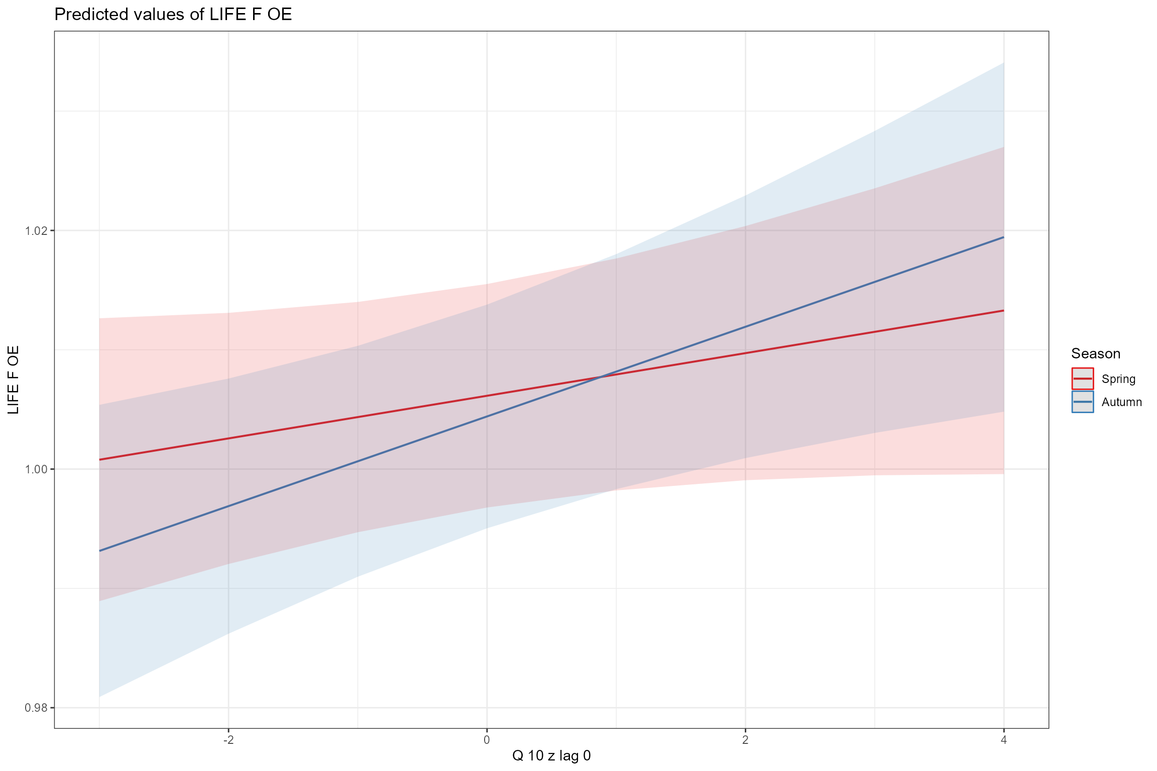
sjPlot::plot_model(model = cs2_mod1,
                   type = "pred",
                   terms = c("Q95z_lag0", "HQA [35, 50, 65]"))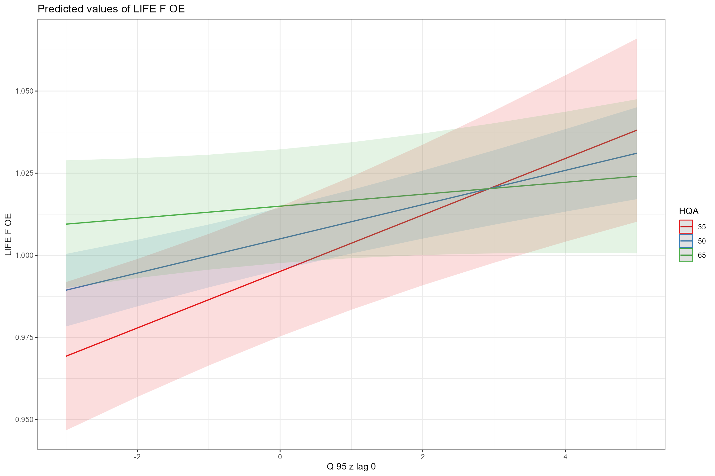
- Finally, the mixed-effects estimates of the time trend at each site
can be extracted and plotted. For reference, the vertical dashed blue
line is the global slope (i.e. the average time trend of 0.001 per year
- see the output from
summary()above). This shows that, after accounting for interannual variation in flow, the majority of sites display a trend of increasing LIFE O:E ratios over time, but that a minority of sites have a decreasing trend.
cs2_mod.coef <- coef(cs2_mod1)[[1]]

cs2_mod.coef$biol_site_id <- as.character(row.names(cs2_mod.coef))

ggplot(cs2_mod.coef, aes(x = biol_site_id, y = Year_cen)) +
  geom_point(colour = "orange")+
  coord_flip() +
  geom_hline(yintercept = 0, linetype = "dashed", colour = "black") +
  geom_hline(yintercept = 0.0011, linetype = "dashed", colour = "blue")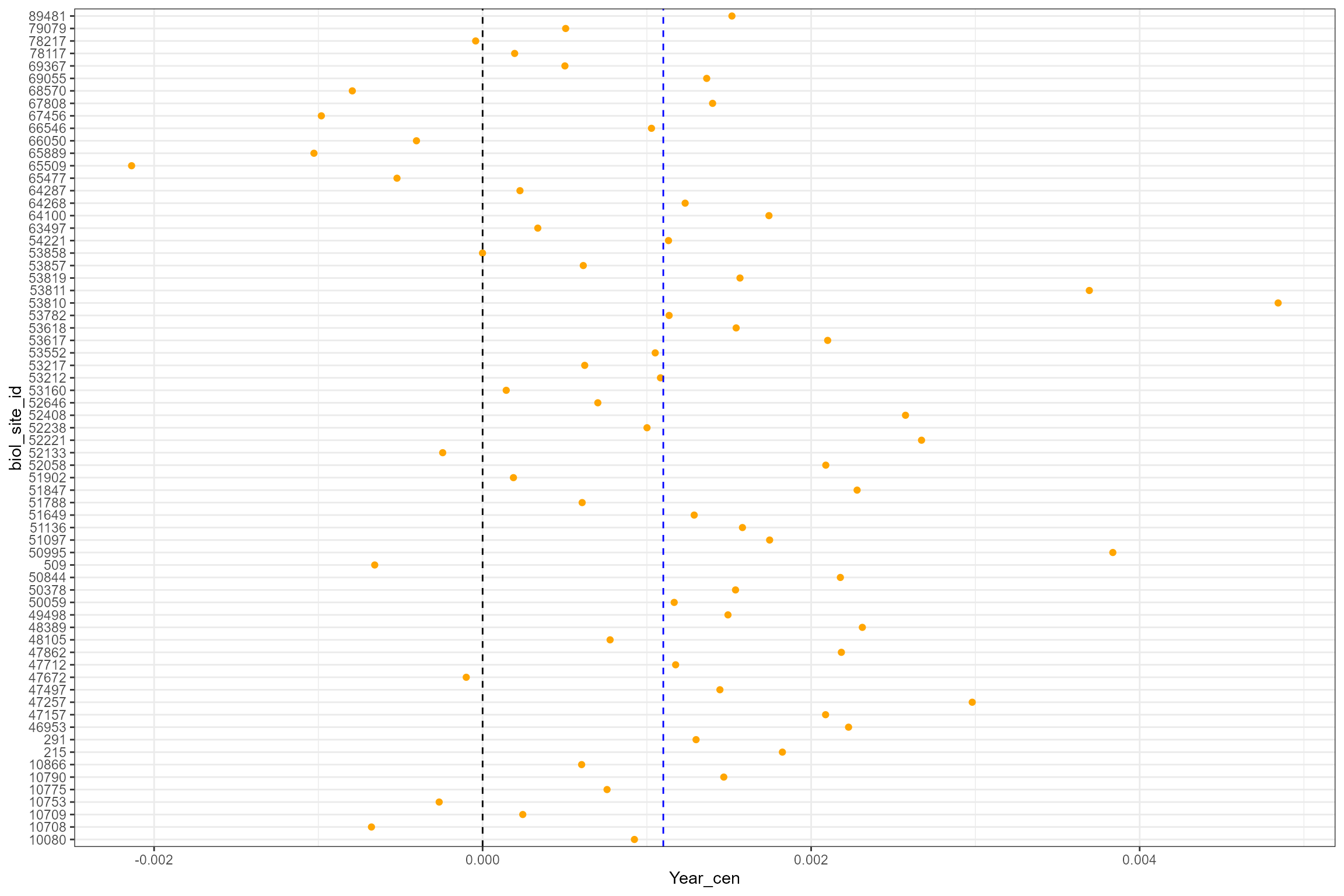
Generalised Additive Model
In addition to a linear model, we also demonstrate how you may apply a generalised additive model for analysis of hydroecological data.
Hierarchical Generalised Additive Models (HGAMs), implemented using the mgcv library were used to model spatial and temporal variation in LIFE O:E. HGAMs allow relationships between the explanatory variables and the response to be described by smooth curves or linear terms (Wood, 2017), whilst also incorporating terms to represent unexplained site-to-site variation (Pedersen et al., 2019). By flexibly describing non-linear relationships nonparametrically, without making a priori assumptions about the form of the relationship, HGAMs can be a suitable alternative to more simple, less flexible linear models.
Linear models 1 and 2 were re-fitted using the gam()
function from mgcv. The same explanatory variables and interaction terms
were tested, but incorporated into the gam() model
structure. The mixture of continuous and categorical predictors was
included within the full models as fixed effects, with continuous
predictors fitted as smoothed terms (using the s()
notation).
To model interactions of continuous variables, the functions,
te() and ti(), can be used. The function
te() is applicable when variables are not on the same
scale, and when interactions include main effects. The function
ti() is used for modelling interaction surfaces that do not
include the main effects, under the assumption that they will be
included separately. In models 1 and 2, below, interactions between two
smoothed terms (i.e Q95z_lag0 * HQA, or Q95z_lag0 * HMSRBB) were
therefore specified using the notation ti(), so the main
effects could be evaluated separately from the interaction term.
In addition, a ‘factor-smooth’ term (Pedersen et al. 2019) was used to model random site-specific intercepts and time trends; the inclusion of a ‘factor-smooth’ term allowed the temporal trend to vary from site to site, and is specified in place of the random effects included within the linear model structures.
Candidate Models:
Model 1
# model 1 (includes interactions)
cs2_gam1 <- mgcv::gam(LIFE_F_OE ~
                     Season +
                     s(Year_cen) +
                     s(Q10z_lag0) +
                     s(Q95z_lag0) +
                     s(Q10z_lag0, by = Season, m = 1) +
                     s(HQA) +
                     s(HMSRBB) +
                     ti(Q95z_lag0, HQA) +
                     #ti(Q95z_lag0, HMSRBB) +
                     s(Year_cen, biol_site_id, bs = "fs"),
                    data = cs2_HE1,
                    #select = TRUE,
                    method = 'REML')

#saveRDS(cs2_gam1, "data/cs2_gam1.RDS")
summary(cs2_gam1)##
## Family: gaussian
## Link function: identity
##
## Formula:
## LIFE_F_OE ~ Season + s(Year_cen) + s(Q10z_lag0) + s(Q95z_lag0) +
## s(Q10z_lag0, by = Season, m = 1) + s(HQA) + s(HMSRBB) + ti(Q95z_lag0,
## HQA) + s(Year_cen, biol_site_id, bs = "fs")
##
## Parametric coefficients:
## Estimate Std. Error t value Pr(>|t|)
## (Intercept) 1.004594 0.004370 229.875 <2e-16 ***
## SeasonAutumn -0.001615 0.001589 -1.016 0.31
## ---
## Signif. codes: 0 '***' 0.001 '**' 0.01 '*' 0.05 '.' 0.1 ' ' 1
##
## Approximate significance of smooth terms:
## edf Ref.df F p-value
## s(Year_cen) 3.897e+00 4.785 7.751 1.69e-06 ***
## s(Q10z_lag0) 1.621e+00 1.981 2.514 0.0687 .
## s(Q95z_lag0) 1.001e+00 1.002 15.533 8.51e-05 ***
## s(Q10z_lag0):SeasonSpring 7.622e-04 8.000 0.000 0.9880
## s(Q10z_lag0):SeasonAutumn 2.886e+00 8.000 0.782 0.0327 *
## s(HQA) 1.000e+00 1.000 0.070 0.7915
## s(HMSRBB) 3.227e+00 3.282 3.179 0.0121 *
## ti(Q95z_lag0,HQA) 1.002e+00 1.003 3.752 0.0529 .
## s(Year_cen,biol_site_id) 1.205e+02 553.000 3.289 < 2e-16 ***
## ---
## Signif. codes: 0 '***' 0.001 '**' 0.01 '*' 0.05 '.' 0.1 ' ' 1
##
## R-sq.(adj) = 0.637 Deviance explained = 67.1%
## -REML = -2863.8 Scale est. = 0.00089614 n = 1467Model 2
# model 2 (includes interactions)
cs2_gam2 <- mgcv::gam(LIFE_F_OE ~
                     Season +
                     s(Year_cen) +
                     s(Q10z_lag0) +
                     s(Q95z_lag0) +
                     s(Q10z_lag0, by = Season, m = 1) +
                     s(HQA) +
                     s(HMSRBB) +
                     #ti(Q95z_lag0, HQA) +
                     ti(Q95z_lag0, HMSRBB) +
                     s(Year_cen, biol_site_id, bs = "fs"),
                    data = cs2_HE1,
                    #select = TRUE,
                    method = 'REML')

#saveRDS(cs2_gam2, "data/cs2_gam2.RDS")
summary(cs2_gam2)##
## Family: gaussian
## Link function: identity
##
## Formula:
## LIFE_F_OE ~ Season + s(Year_cen) + s(Q10z_lag0) + s(Q95z_lag0) +
## s(Q10z_lag0, by = Season, m = 1) + s(HQA) + s(HMSRBB) + ti(Q95z_lag0,
## HMSRBB) + s(Year_cen, biol_site_id, bs = "fs")
##
## Parametric coefficients:
## Estimate Std. Error t value Pr(>|t|)
## (Intercept) 1.004458 0.004375 229.57 <2e-16 ***
## SeasonAutumn -0.001510 0.001590 -0.95 0.342
## ---
## Signif. codes: 0 '***' 0.001 '**' 0.01 '*' 0.05 '.' 0.1 ' ' 1
##
## Approximate significance of smooth terms:
## edf Ref.df F p-value
## s(Year_cen) 3.969e+00 4.871 7.917 1.10e-06 ***
## s(Q10z_lag0) 1.648e+00 2.017 2.766 0.0645 .
## s(Q95z_lag0) 1.004e+00 1.007 15.449 8.81e-05 ***
## s(Q10z_lag0):SeasonSpring 1.129e-03 8.000 0.000 0.9793
## s(Q10z_lag0):SeasonAutumn 2.894e+00 8.000 0.784 0.0324 *
## s(HQA) 1.001e+00 1.001 0.064 0.8001
## s(HMSRBB) 3.203e+00 3.257 3.222 0.0117 *
## ti(Q95z_lag0,HMSRBB) 2.369e+00 3.292 0.975 0.4633
## s(Year_cen,biol_site_id) 1.199e+02 553.000 3.264 < 2e-16 ***
## ---
## Signif. codes: 0 '***' 0.001 '**' 0.01 '*' 0.05 '.' 0.1 ' ' 1
##
## R-sq.(adj) = 0.637 Deviance explained = 67.1%
## -REML = -2862.9 Scale est. = 0.00089689 n = 1467
Similar to the linear models, we use model_cv to compare
the two candidate GAMs fitted above. model_cv performs
repeated, stratified k-fold cross-validation, which can be used to
evaluate a model’s ability to predict the response at sites in the
calibration dataset. Predictive performance is measured using the Root
Mean Square Error (RMSE); lower values indicate better predictions. r is
set at 10 to give stable RMSE estimates and control is used to help
prevent model convergence issues.
# my_control = lmerControl(optimizer="bobyqa", optCtrl = list(maxfun = 10000))

# Model 1
# cs2_cv_gam1 <- hetoolkit::model_cv(model = cs2_gam1,
#                               data = cs2_HE1,
#                               group = "biol_site_id",
#                               k = 5,
#                               r = 10,
#                               control = my_control)

# Model 2
# cs2_cv_gam2 <- hetoolkit::model_cv(model = cs2_gam2,
#                               data = cs2_HE1,
#                               group = "biol_site_id",
#                               k = 5,
#                               r = 10,
#                               control = my_control)
RMSE is very similar for both models, and is only marginally lower for model 1.
# Let's compare the RMSE results
cs2_cv_gam1[[1]]
## [1] 0.0320489
cs2_cv_gam2[[1]]## [1] 0.03220954In this instance, we also compared the Akaike Information Criterion (AIC) of model 1 and model 2. AIC is a relative measure of how well a model fits a set of data. A lower AIC value indicates a better-fitting model. Model 2 has a notably lower AIC, compared to model 1.
Model 2 was therefore chosen as the final model.
# Let's compare the AIC
AIC(cs2_gam1, cs2_gam2)
## df AIC
## cs2_gam1 148.3365 -5978.648
## cs2_gam2 152.6252 -5969.834Model interpretation
The final model (model 2) included the fixed predictors
Q10z_lag0, Q95z_lag0, Season,
HQA, Year_cen, and HMSRBB, plus
two interaction terms, and a factor-smooth term that allowed the
temporal trend to vary from site-to-site.
On average, LIFE O:E was lower in autumn than spring. LIFE O:E decreased with the extent of habitat modification (HMSRBB score), with the steepest decrease in LIFE O:E observed when HMSRBB was greater than 20, and habitat quality (HQA) demonstrated a weak positive relationship with LIFE O:E. There was also an underlying long-term increasing trend across all sites (Year_cen); however, in contrast to the linear model, the HGAM found that LIFE O:E scores peaked in ~2005, and decreased slightly after this - although more recent temporal change (~2010-onwards) in LIFE O:E is associated with a higher degree of uncertainty.
After controlling for these influences, LIFE O:E was positively
associated with the Q95z flow in the preceding six month winter or
summer period and to a lesser extent with the Q10z flow, similar to the
linear model. While Q95z demonstrated a linear relationship with LIFE
O:E, Q10z demonstrated a slightly non-linear relationship, and LIFE O:E
gradually plateaued at the highest antecedent flows; however, at the
highest antecedent flows, the flow-ecology relationship was associated
with a higher degree of uncertainty. The effect of Q10z was stronger in
autumn than in spring (s(Q10z_lag0, by = season)
interaction).
The effect of Q95z was strongest at sites with a high HMSRBB score
(ti(Q95z_lag0, HMSRBB) interaction), indicating that
macroinvertebrate communities at sites with more modified habitat were
more sensitive to antecedent low flows, while sites with more natural
habitat demonstrated lesser sensitivity to change in antecedent flow. At
modified sites, LIFE O:E was positively associated with the Q95z flow in
the preceding six months, whereas at sites with a lesser degree of
modification, LIFE O:E remained relatively unchanged regardless of
antecedent flow conditions. However, the magnitude of change in LIFE O:E
associated with the interaction term
(ti(Q95z_lag0, HMSRBB)) was weaker when compared to the
individual fixed effects (s(Q95z_lag0) and
s(HMSRBB)); with LIFE O:E showing a maximum change of ~0.01
for the interaction term, and a maximum change of ~0.03 and ~0.1 for the
Q95z and HMSRBB main effects, respectively.
The factor-smooth estimates showed a relatively large variance in the intercept among the 68 sites, indicating a high degree of spatial variation.
gratia::draw(cs2_gam2, residuals = TRUE) &
  plot_annotation(caption = paste("Deviance explained:", round((summary(cs2_gam2)$dev)*100, digits = 1),"%"))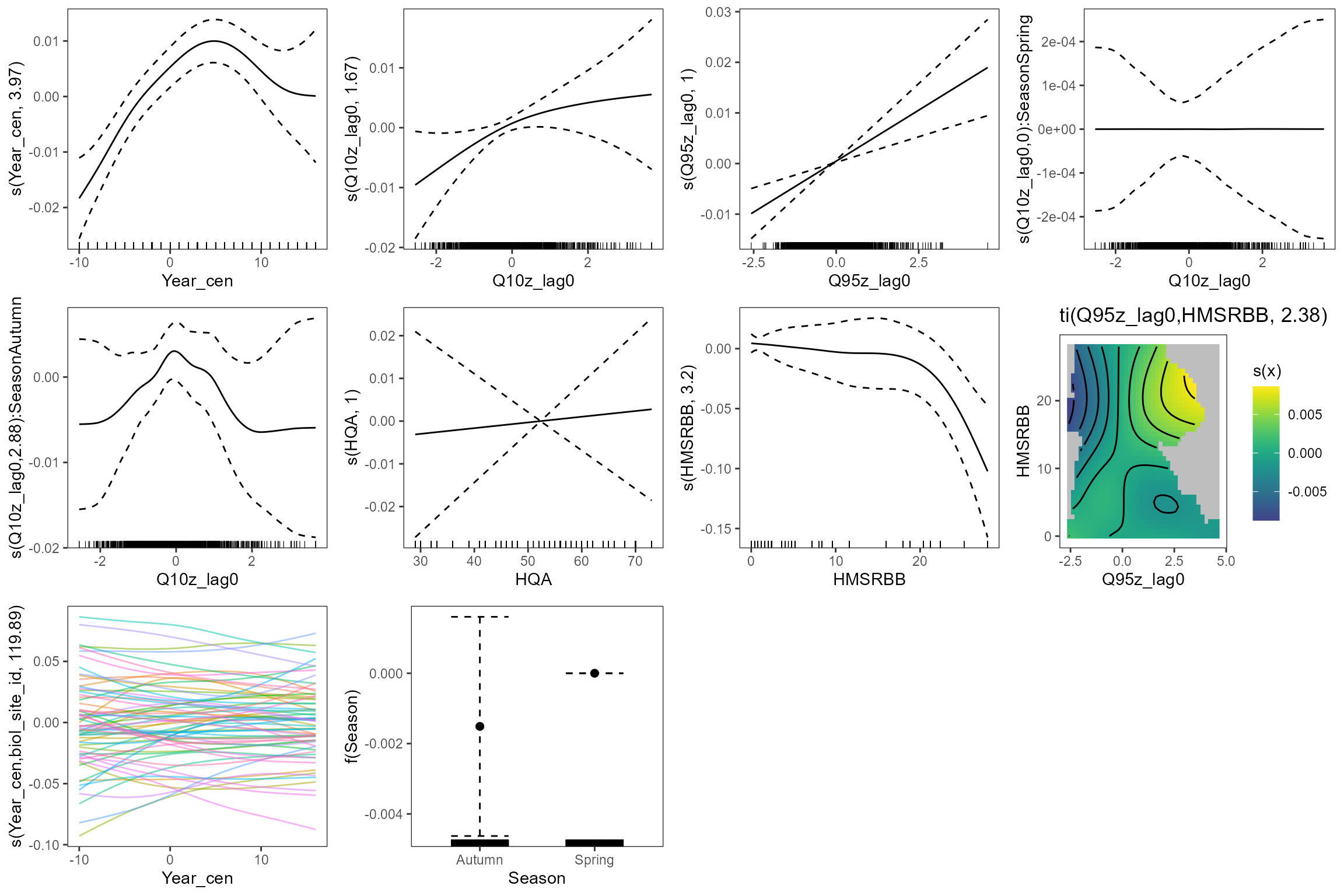
summary(cs2_gam2)##
## Family: gaussian
## Link function: identity
##
## Formula:
## LIFE_F_OE ~ Season + s(Year_cen) + s(Q10z_lag0) + s(Q95z_lag0) +
## s(Q10z_lag0, by = Season, m = 1) + s(HQA) + s(HMSRBB) + ti(Q95z_lag0,
## HMSRBB) + s(Year_cen, biol_site_id, bs = "fs")
##
## Parametric coefficients:
## Estimate Std. Error t value Pr(>|t|)
## (Intercept) 1.004458 0.004375 229.57 <2e-16 ***
## SeasonAutumn -0.001510 0.001590 -0.95 0.342
## ---
## Signif. codes: 0 '***' 0.001 '**' 0.01 '*' 0.05 '.' 0.1 ' ' 1
##
## Approximate significance of smooth terms:
## edf Ref.df F p-value
## s(Year_cen) 3.969e+00 4.871 7.917 1.10e-06 ***
## s(Q10z_lag0) 1.648e+00 2.017 2.766 0.0645 .
## s(Q95z_lag0) 1.004e+00 1.007 15.449 8.81e-05 ***
## s(Q10z_lag0):SeasonSpring 1.129e-03 8.000 0.000 0.9793
## s(Q10z_lag0):SeasonAutumn 2.894e+00 8.000 0.784 0.0324 *
## s(HQA) 1.001e+00 1.001 0.064 0.8001
## s(HMSRBB) 3.203e+00 3.257 3.222 0.0117 *
## ti(Q95z_lag0,HMSRBB) 2.369e+00 3.292 0.975 0.4633
## s(Year_cen,biol_site_id) 1.199e+02 553.000 3.264 < 2e-16 ***
## ---
## Signif. codes: 0 '***' 0.001 '**' 0.01 '*' 0.05 '.' 0.1 ' ' 1
##
## R-sq.(adj) = 0.637 Deviance explained = 67.1%
## -REML = -2862.9 Scale est. = 0.00089689 n = 1467Model diagnostics
We can run gam.check(), which produces some diagnostic
information about the fitting procedure and results. The default is to
produce 4 residual plots, some information about the convergence of the
smoothness selection optimisation, and to run diagnostic tests of
whether the basis dimension choices are adequate. Below we run
gam.check() for Model 2, as it had the lowest RMSE score,
to produce four diagnostic plots.
These include:
Q-Q Plot. This plots two sets of quantiles against one another. If the residuals fall along a roughly straight line at a 45-degree angle, then the residuals are roughly normally distributed. We can see in our Q-Q plot below that the residuals tend to deviate from the 45-degree line on the tail ends, which could be an indication that they’re not normally distributed.
Residuals vs linear pred. This plot checks the assumption of homogeneous variances, which states that the error variance should be constant regardless of what value the response takes. Here we can see that the residuals generally have a similar amount of vertical scatter at all fitted values of the response, with some deviation at lower values of the linear predictor.
Histogram of residuals. This is an alternative to plot 2 for verifying the assumption of normally distributed errors. Here we can see that the probability distribution of the model residuals is reasonably similar to a normal distribution.
Response vs fitted values. This plot shows the relationship between the fitted (predicted) and observed (true) values of the response variable. If the model fits the data well, the points should be clustered around the diagonal 1:1 line, which represents a perfect fit (fitted=observed). Here we can see the model provides a reasonably good fit to the data, but with the weakest predictive power at low LIFE O:E values (observed values).
gam.check(cs2_gam2)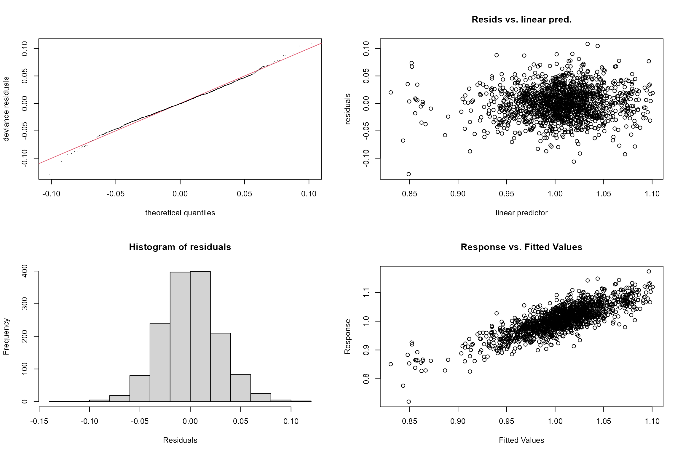
##
## Method: REML   Optimizer: outer newton
## full convergence after 9 iterations.
## Gradient range [-0.0006127483,0.00128728]
## (score -2862.869 & scale 0.000896886).
## Hessian positive definite, eigenvalue range [0.0002265474,731.3445].
## Model rank =  749 / 749
##
## Basis dimension (k) checking results. Low p-value (k-index<1) may
## indicate that k is too low, especially if edf is close to k'.
##
##                                 k'      edf k-index p-value
## s(Year_cen)               9.00e+00 3.97e+00    0.92  <2e-16 ***
## s(Q10z_lag0)              9.00e+00 1.65e+00    0.94   0.005 **
## s(Q95z_lag0)              9.00e+00 1.00e+00    0.96   0.065 .
## s(Q10z_lag0):SeasonSpring 8.00e+00 1.13e-03    0.94   0.010 **
## s(Q10z_lag0):SeasonAutumn 8.00e+00 2.89e+00    0.94   0.010 **
## s(HQA)                    9.00e+00 1.00e+00    0.99   0.310
## s(HMSRBB)                 9.00e+00 3.20e+00    0.98   0.220
## ti(Q95z_lag0,HMSRBB)      1.60e+01 2.37e+00    0.98   0.195
## s(Year_cen,biol_site_id)  6.70e+02 1.20e+02    0.92   0.010 **
## ---
## Signif. codes:  0 '***' 0.001 '**' 0.01 '*' 0.05 '.' 0.1 ' ' 1
In addition to the diagnostic plots, gam.check() returns
a check of the basis dimensions (k) of smoothed terms that were included
within model 2. This can also be returned by running
k.check(). For model 2 above, the basis dimensions (k) are
set at the default values of mgcv::gam().
Above, the gam.check() report returned low p-values (and
k-index <1) for the Q10_lag0 and Year_cen variables, and their
interactions. These results indicate that k may be too low, especially
where the EDF (effective degrees of freedom) are close to their maximum
possible value (k’), meaning that the wiggliness of the model may be
overly constrained by the default k, and the model could fit the data
better (with greater wiggliness) if k were to be increased. In other
words, the trade off between smoothness and wiggliness is not balanced.
The model was first refitted with larger k values (k = 20) for Q10_lag0
and Year_cen variables (below).
Re-running k.check() on the adjusted model demonstrated some increase in p-values, but these remained reasonably low for the Q10z_lag0 and Year_cen variables. However, applying k=20 only marginally increased the EDF for the Q10z_lag0 and Year_cen variables. A second adjusted model, applying k=30 for Q10z_lag0 and k=25 for Year_cen, was also trialed and, again, only marginal increases in the EDF were observed. To balance computational time, and model wiggliness, a k value of 20 was therefore applied for Q10z_lag0 and Year_cen variables. Using this model, we can see that the EDF are no longer close to k’.
In case it is not clear from the above, note that k, k-index and k’ denote (somewhat confusingly) slightly different things. See Pedersen et al. (2019; https://doi.org/10.7717/peerj.6876) or Wood (2017; https://www.taylorfrancis.com/books/mono/10.1201/9781315370279/generalized-additive-models-simon-wood) for further information on this and other aspects of GAMs.
Adjust k-values:
Model 2_k20
cs2_gam2_k20 <- mgcv::gam(LIFE_F_OE ~
                     Season +
                     s(Year_cen, k = 20) +
                     s(Q10z_lag0, k = 20) +
                     s(Q95z_lag0) +
                     s(Q10z_lag0, by = Season, m = 1, k = 20) +
                     s(HQA) +
                     s(HMSRBB) +
                     #ti(Q95z_lag0, HQA) +
                     ti(Q95z_lag0, HMSRBB) +
                     s(Year_cen, biol_site_id, bs = "fs"),
                    data = cs2_HE1,
                    #select = TRUE,
                    method = 'REML')


#saveRDS(cs2_mod2_k20, "vignettes/data/cs2_mod2_k20.RDS")
mgcv::k.check(cs2_gam2_k20)## k' edf k-index p-value
## s(Year_cen) 19 4.111071e+00 0.9234973 0.0000
## s(Q10z_lag0) 19 1.743350e+00 0.9367064 0.0075
## s(Q95z_lag0) 9 1.001291e+00 0.9575204 0.0375
## s(Q10z_lag0):SeasonSpring 19 1.125498e-03 0.9367064 0.0150
## s(Q10z_lag0):SeasonAutumn 19 3.089237e+00 0.9367064 0.0150
## s(HQA) 9 1.000048e+00 0.9865052 0.2675
## s(HMSRBB) 9 3.204170e+00 0.9759994 0.1975
## ti(Q95z_lag0,HMSRBB) 16 2.397526e+00 0.9900978 0.3325
## s(Year_cen,biol_site_id) 670 1.198629e+02 0.9234973 0.0025Model 2_k30
cs2_gam2_k50 <- mgcv::gam(LIFE_F_OE ~
                     Season +
                     s(Year_cen, k = 25) +
                     s(Q10z_lag0, k = 30) +
                     s(Q95z_lag0) +
                     s(Q10z_lag0, by = Season, m = 1, k = 30) +
                     s(HQA) +
                     s(HMSRBB) +
                     #ti(Q95z_lag0, HQA) +
                     ti(Q95z_lag0, HMSRBB) +
                     s(Year_cen, biol_site_id, bs = "fs"),
                    data = cs2_HE1,
                    #select = TRUE,
                    method = 'REML')

#saveRDS(cs2_mod2_k50, "vignettes/data/cs2_mod2_k50.RDS")
## k' edf k-index p-value
## s(Year_cen) 24 4.111938e+00 0.9233217 0.0000
## s(Q10z_lag0) 29 1.775009e+00 0.9366479 0.0100
## s(Q95z_lag0) 9 1.001641e+00 0.9574724 0.0400
## s(Q10z_lag0):SeasonSpring 29 2.861593e-03 0.9366479 0.0075
## s(Q10z_lag0):SeasonAutumn 29 3.086118e+00 0.9366479 0.0050
## s(HQA) 9 1.000051e+00 0.9865631 0.2600
## s(HMSRBB) 9 3.203737e+00 0.9760505 0.1750
## ti(Q95z_lag0,HMSRBB) 16 2.400775e+00 0.9905168 0.2950
## s(Year_cen,biol_site_id) 670 1.198543e+02 0.9233217 0.0000