Macroinvertebrates in chalk streams
Environment Agency / APEM Ltd
05 December, 2025
CaseStudy1.RmdIntroduction
This case study focuses on a macroinvertebrate dataset of 33 sampling locations on the Test and Itchen (T&I), two groundwater-fed Chalk rivers in Hampshire, England. In particular, it illustrates the use of water quality data and modelled flow data within a hydro-ecological model.
Sites were included in the model calibration dataset if they met all of the following criteria:
- At least 10 macroinvertebrate samples (spanning at least 5 years) within the time period covered by the flow data.
- The site is not on a side channel where flow is controlled by hatches/sluices.
- The site is located on a reach with perennial flow (defined as natural Q99 > 0).
- The site can be paired with a suitably-located River Habitat Survey (RHS) site.
- The site is not subject to overwhelming artificial physical modifications (e.g. dredged channel, close upstream weir).
- The site has no major water quality issues.
- The site is not subject to some other, potentially over-riding, pressure.
- Signal crayfish are absent.
- The site has no history of major habitat restoration work.
Historical flows at each sampling location were modelled using the EA’s T&I regional groundwater model. Naturalised flows were also modelled by turning off the effect of abstraction and discharges. Using these two flow time series, the case study explores if and how the macroinvertebrate community (as indexed by LIFE O:E ratios) is affected long-term flow alteration, whilst also controlling for natural hydrological variability (flow history) and changes in water quality.
As this case study is intended to illustrate the application of the HE toolkit, rather than be a comprehensive analysis in its own right, some of the analytical steps have been simplified for brevity.
This case study is optimised for viewing in Chrome.
Set-up
Install and load the HE Toolkit:
#install.packages("remotes")
library(remotes)
# Conditionally install hetoolkit from github
if ("hetoolkit" %in% installed.packages() == FALSE) {
remotes::install_github("APEM-LTD/hetoolkit")
}
library(hetoolkit)Install and load the other packages necessary for this case study:
Metadata
We start by importing a “metadata” file with the following columns:
- biol_site_id = Macroinvertebrate sampling site ids;
- flow_site_id = river reach id;
- wq_site_id = water quality site id; and
- rhs_survey_id = river habitat survey (RHS) ids (survey ids not site id, in case multiple surveys have been undertaken at a site).
These id’s are used below to download data from the Environment Agency’s (EA) Ecology and Fish Data Explorer (EDE), Water Quality Archive, and Defra’s data.gov.uk website, and to join disparate data sets together.
# Import metadata file containing site id's
cs1_metadata <- readxl::read_excel("Data/CaseStudy1/cs1_metadata.xlsx", col_types = "text") %>%
dplyr::rename(flow_site_id = reach_id)
# Get site lists, for use with functions
cs1_biolsites <- cs1_metadata$biol_site_id
cs1_rhssurvey <- cs1_metadata$rhs_survey_id
cs1_flowsites <- cs1_metadata$flow_site_id
cs1_wqsites <- cs1_metadata$wq_site_idRiver Habitat Survey (RHS) data
The import_rhs function downloads River Habitat Survey
(RHS) data from Open Data. Below, we use our list
cs1_rhssurveys to filter the downloaded data. We use the
select function to filter the two variables in the RHS data set that we
will need for the data analysis: the site id and the bank and bed
re-sectioning sub-score (HMSRBB), where higher scores represent greater
channel modification. We rename the Survey ID to rhs_survey_id to fit
the standardised column names used throughout the hetoolkit case
studies.
# Import open-source RHS survey data
cs1_rhs_data <- hetoolkit::import_rhs(surveys = cs1_rhssurvey)
# Rename survey.id as rhs_survey_id to facilitate later data joining
cs1_rhs_data <- cs1_rhs_data %>%
dplyr::rename(rhs_survey_id = Survey.ID,
HMSRBB = Hms.Rsctned.Bnk.Bed.Sub.Score) %>%
# Use select function in dplyr to select the two columns we need
dplyr::select(rhs_survey_id, HMSRBB)Look at the RHS data:
Environmental data
## Import environmental data
The import_env function downloads environmental data
from the Environment Agency’s Ecology and Fish Data Explorer (EDE).
Below, we use our list cs1_biolsites to filter the data
from EDE.
# Import biology data from EDE
cs1_env_data <- hetoolkit::import_env(sites=cs1_biolsites)View the environment data:
Map sites
To make a map of the sample sites, we use the environmental base data
that we have downloaded from the Ecology and Fish Data Explorer using
import_env, this gives us their NGRs. We translate the NGRs
to full latitude / longitude (WGS84) and match this back to the env_data
so we have information to include in the plot.
Finally we use leaflet to plot the points indicating the
sample sites. The points are labelled with the biology sample site ID,
the EA area code and catchment.
# Convert national grid ref (NGR) to full lat / long from env_data (from import_env function)
# WGS84 is lat/long.
temp.eastnorths <- rnrfa::osg_parse(cs1_env_data$NGR_10_FIG, coord_system = "WGS84") %>% as_tibble()
## match to back to env data to give details on map.
cs1_env_data_map <- cbind(cs1_env_data, temp.eastnorths) %>%
dplyr::select(AGENCY_AREA, WATER_BODY, CATCHMENT, WATERBODY_TYPE, biol_site_id, lat, lon) %>%
dplyr::mutate(label = paste0("<b>", as.character(biol_site_id), "</b><br/>",
AGENCY_AREA, "<br/>", CATCHMENT))
## Create map
leaflet() %>%
leaflet::addTiles() %>%
leaflet::addMarkers(lng = cs1_env_data_map$lon, lat = cs1_env_data_map$lat,
popup = cs1_env_data_map$label,
options = popupOptions(closeButton = FALSE))Assess site similarity
Prior to building a hydro-ecological model, it is helpful to identify
any sites that could be an outlier because they are physically
dissimilar to the other sites. The plot_sitepca function
performs a Principal Components Analysis (PCA), which reduces site-level
environmental variables to uncorrelated principal components. The
relative importance of the environmental variables are expressed by
arrow length, and sites that are plotted more closely together have more
similar environmental components. The first principal component (PC1) is
plotted on the horizontal axis, as it represents the most dominant
source of variation in the dataset. Hence, we can use this to identify
sites that may be outliers as they will be plotted in isolation from
other sites.
# plot site PCA
hetoolkit::plot_sitepca(data = cs1_env_data,
vars = c("ALTITUDE", "SLOPE", "WIDTH", "DEPTH",
"BOULDERS_COBBLES", "PEBBLES_GRAVEL", "SILT_CLAY"),
eigenvectors = TRUE, label_by = "biol_site_id") 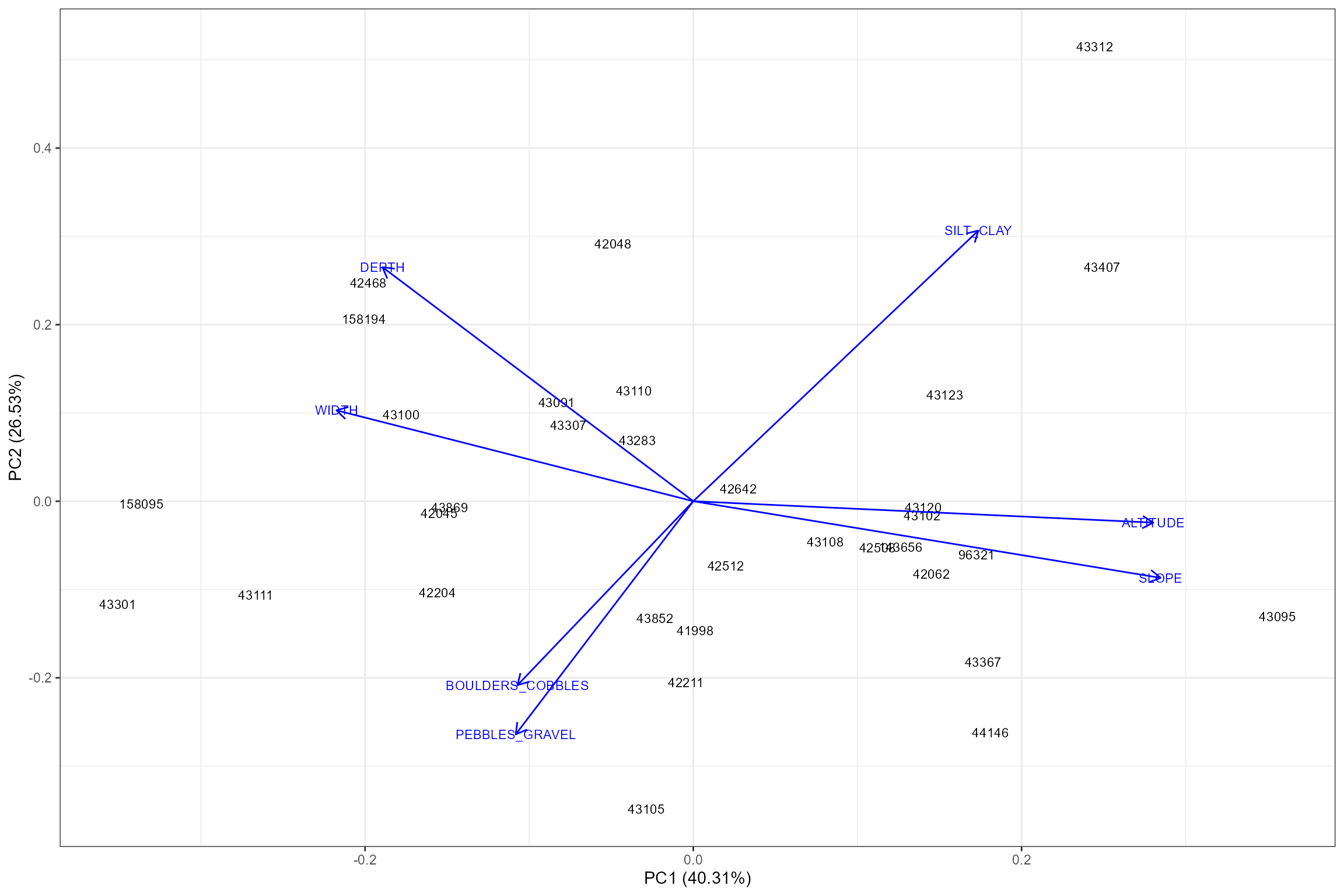
The PCA plot indicates that site 43312 has an unusually high (68%) percentage of silt/clay substrate compared to the other sites, but after checking the environmental data table above we decide to leave it in the calibration dataset.
Predict expected indices
The predict_indices function mirrors the functionality
of the RICT2 model, by using the environmental data downloaded from the
EDE to generate expected scores under minimally impacted reference
conditions. To run the predict_indices function, the data
must not contain any NA’s:
# Check for missing substrate data (none in this dataset)
cs1_env_data %>%
dplyr::select(BOULDERS_COBBLES, PEBBLES_GRAVEL, SAND, SILT_CLAY) %>%
summarise_all(~sum(is.na(.)))## # A tibble: 1 × 4
## BOULDERS_COBBLES PEBBLES_GRAVEL SAND SILT_CLAY
## <int> <int> <int> <int>
## 1 0 0 0 0Having checked that substrate data is complete, we now calculate the
expected scores using the predict_indices. We calculate all
of the indices and then filter these down to the indices we want to use
for this analysis.
# Run the predict function
cs1_predict_data <- hetoolkit::predict_indices(env_data = cs1_env_data, file_format = "EDE")
# Rename and organise the season column
cs1_predict_data <- cs1_predict_data %>%
dplyr::select("biol_site_id", "SEASON", "TL3_LIFE_Fam_DistFam")%>%
dplyr::rename(Season = SEASON) %>%
dplyr::mutate(Season = case_when(Season == 1 ~ "Spring",
Season == 2 ~ "Summer",
Season == 3 ~ "Autumn",
Season == 4 ~ "Winter"))
# Finally, select the variables in the Env data we want to keep
cs1_env_data <- cs1_env_data %>%
dplyr::select(biol_site_id, DIST_FROM_SOURCE, ALTITUDE, SLOPE, WIDTH, DEPTH,
BOULDERS_COBBLES, PEBBLES_GRAVEL, SAND, SILT_CLAY, ALKALINITY)Biology data
Import Macroinvertebrate data
The import_inv function imports macroinvertebrate
sampling data from the EA’s Ecology and Fish Data Explorer. Below, we
use our list cs1_biolsites to filter the data from EDE. We
download data for the period from 1995 (pre-1995 data was excluded as it
was subject to external audit but not an internal analytical quality
control during this time) to the end of the modelled flow period
(2017).
# Download data from EDE with hetoolkit
cs1_biol_data <- hetoolkit::import_inv(source = "parquet", sites = cs1_biolsites,
start_date = "1995-01-01", end_date = "2017-12-31")
# Filter on spring and autumn samples, and select just the variables we want to keep
cs1_biol_data <- cs1_biol_data %>%
dplyr:: filter(Season == "Spring" | Season == "Autumn") %>%
dplyr::select(biol_site_id, SAMPLE_DATE, LIFE_N_TAXA, LIFE_FAMILY_INDEX, LIFE_SCORES_TOTAL,
Month, Season, Year)
cs1_biol_data$biol_site_id <- as.character(cs1_biol_data$biol_site_id)View the macroinvertebrate data:
Calculate O:E ratios
Now we join the observed and expected LIFE scores into a single data frame so that O:E ratios (Observed/Expected) ratios can be calculated. Prior to joining the biology data with other datasets, it is advisable to remove any replicate or duplicate samples collected from a site within the same year and season.
cs1_biol_data <- cs1_biol_data %>% distinct(biol_site_id, Year, Season, .keep_all = TRUE)
# Join predicted indices to the invertebrate data by id and season
# into a new data frame called cs1_biol_all
cs1_biol_all <- dplyr::left_join(cs1_biol_data, cs1_predict_data, by = c("biol_site_id", "Season"))
# Join the environmental data for later use
cs1_biol_all <- dplyr::left_join(cs1_biol_all, cs1_env_data, by = "biol_site_id")
# Calculate LIFE O:E scores
cs1_biol_all <- cs1_biol_all %>%
mutate(LIFE_F_O = LIFE_FAMILY_INDEX,
LIFE_F_E = TL3_LIFE_Fam_DistFam,
LIFE_F_OE = LIFE_F_O / LIFE_F_E,
date = SAMPLE_DATE) %>%
# Select variables we want to keep
dplyr::select(biol_site_id, Year, Season, Month, date, DIST_FROM_SOURCE, LIFE_F_OE)View all biology data:
Exploratory plots
The exploratory plots below show: * The number of macroinvertebrate samples per site, by season, * The monthly distribution of spring and autumn macroinvertebrate samples; * The distribution of the response variable (LIFE O:E); and * Time series of LIFE O:E ratios at each site.
# Number of macroinvertebrate samples by site & season
ggplot(cs1_biol_all, aes(x = factor(biol_site_id,
levels = rev(levels(factor(biol_site_id)))), fill = Season)) +
geom_bar()+
coord_flip()+
xlab("Site") +
ylab("Number of macroinvertebrate samples")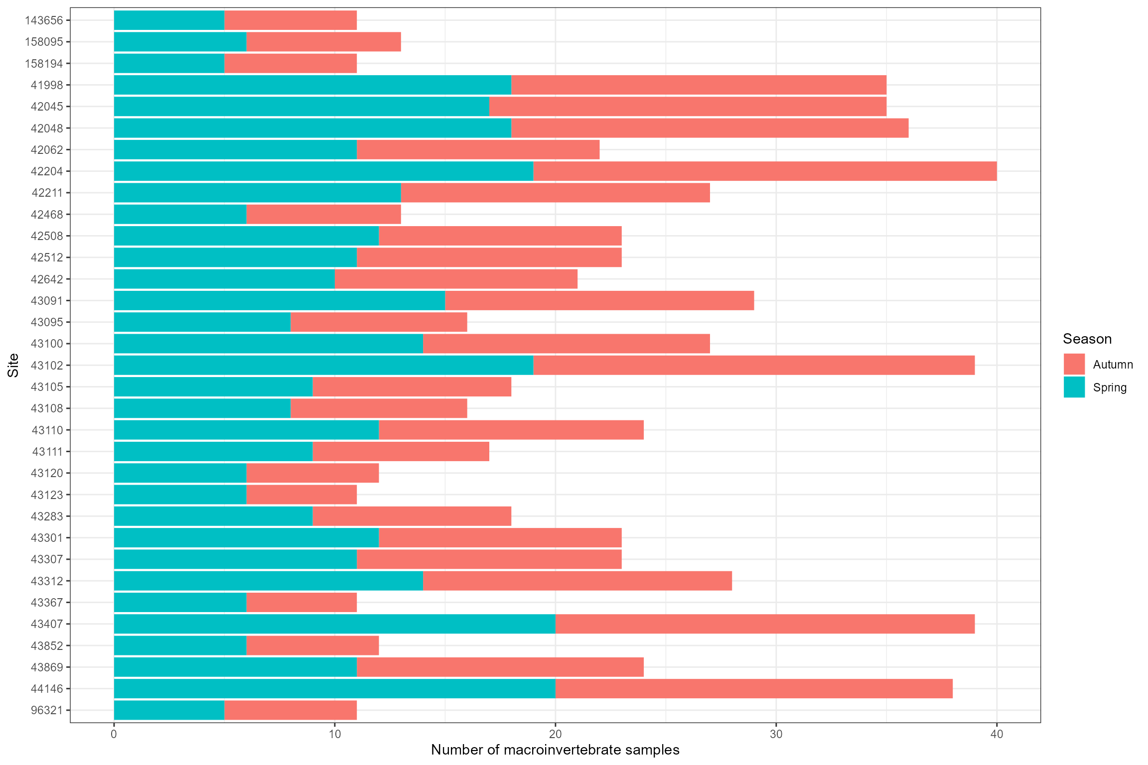
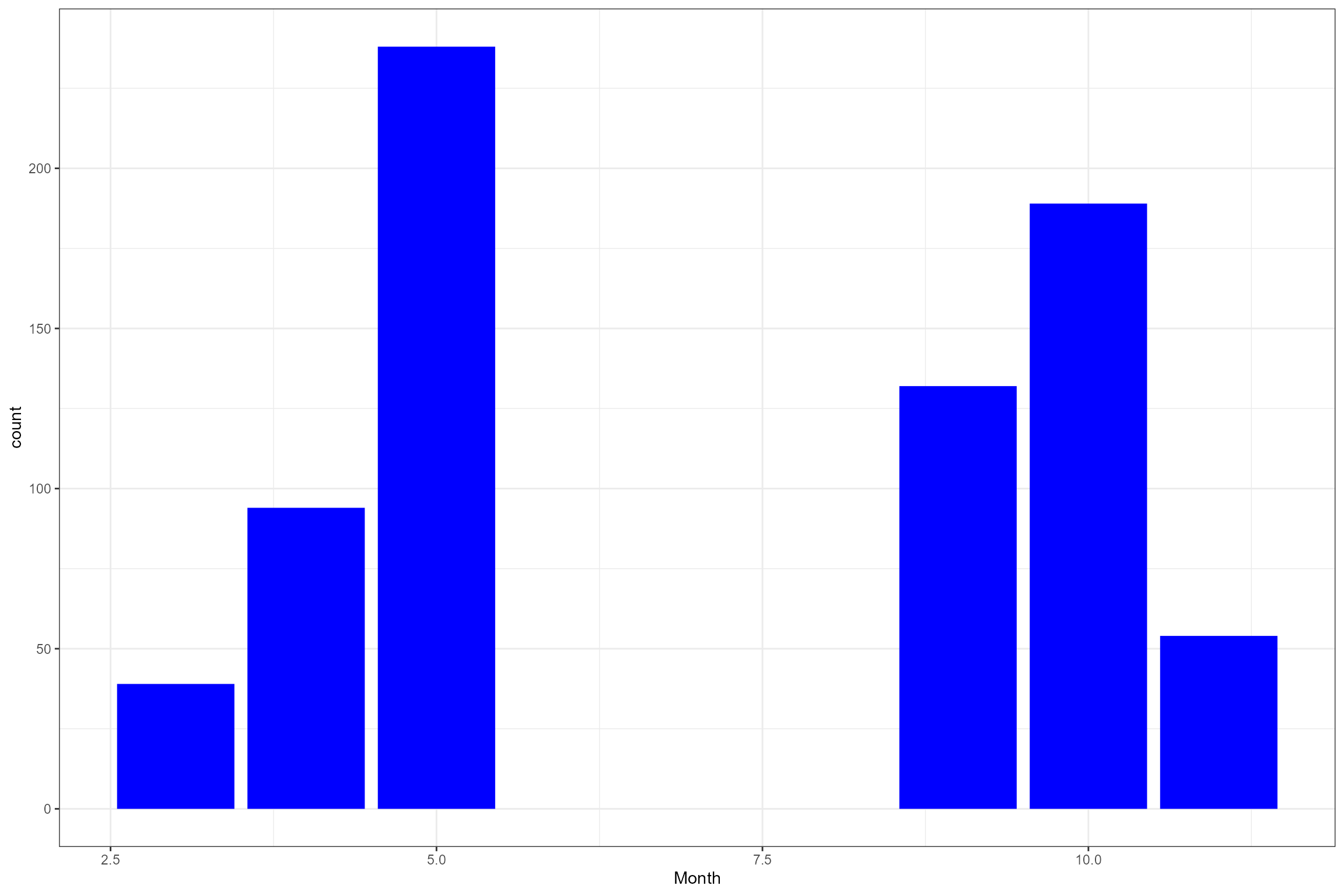
# Histogram of LIFE O:E ratios
ggplot(data = cs1_biol_all, aes(x = LIFE_F_OE)) +
geom_histogram(color="black", fill="grey") +
xlab("LIFE F OE") 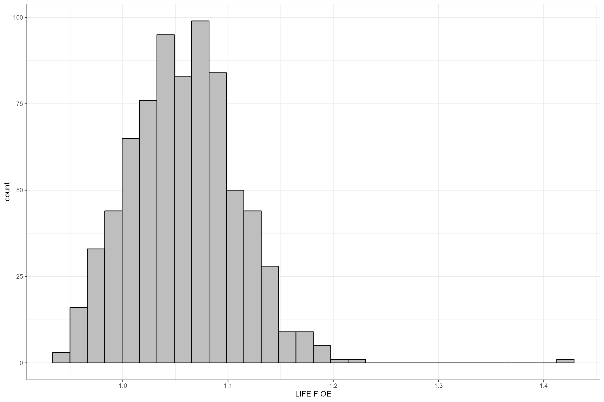
# Time series plots
ggplot(data = cs1_biol_all, aes(x = date, y = LIFE_F_OE)) +
geom_point() +
ylab("LIFE O:E ratio") +
xlab("") +
facet_wrap(~ biol_site_id)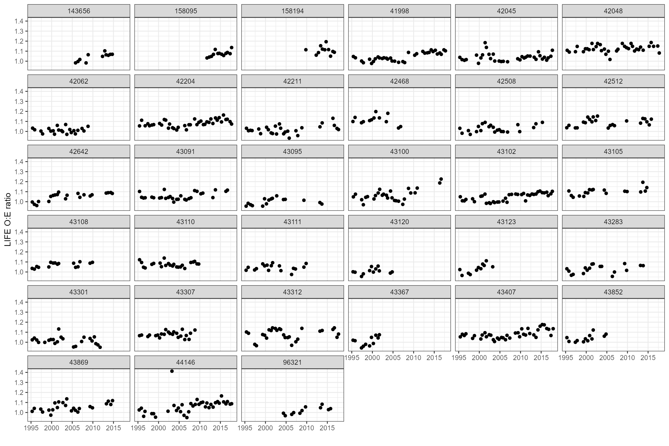
Water quality data
Import water quality data
The import_wq function imports water quality data from
the Environment Agency’s Water Quality Archive database. Below we use
our list cs1_wqsites to import water quality data from 2000
onwards. Note that there are just 25 unique water quality sites linked
to the 33 macroinvertebrate sites. The dets argument is used to import
data for two determinands - Ammoniacal Nitrogen as N (111) and
Orthophosphate, reactive as P (180) - which are useful indicators of
organic pollution and eutrophication.
cs1_wq_data <- hetoolkit::import_wq(sites = cs1_wqsites, dets = c(111, 180), start_date = "2000-01-01")
# import_wq updated November 2025
## Need to re-format outputs, so that it is compatible with workflow
cs1_wq_data <- cs1_wq_data %>%
dplyr::rename(det_label = determinand) %>%
mutate(date = as.Date(date_time)) %>%
mutate(det_label = case_when(det_label == "Ammoniacal Nitrogen as N"
~ "Ammonia(N)",
det_label == "Orthophosphate, reactive as P"
~ "Orthophospht")) %>%
select(wq_site_id, date, det_label, det_id, result, unit)Additional water quality data
The Water Quality Archive database only contains data from 2000 onwards, so below we manually load in 1990-1999 water quality data supplied by the Environment Agency and join it to our imported water quality dataset.
cs1_additional_wq_data <- readRDS("Data/CaseStudy1/cs1_additional_wq.rds")
cs1_wq_data <- rbind(cs1_wq_data,
cs1_additional_wq_data %>% dplyr::select(wq_site_id, date, det_label, det_id, result, unit)) %>%
dplyr::mutate(year = lubridate::year(date)) View all the water quality data:
Summarise water quality
Some sites show strong trends in orthophosphate and ammonia, so time-varying statistics are likely to be more useful than long-term statistics.
# First view data as time series to check for significant step changes or trends
cs1_wq_data %>%
dplyr::filter(det_label == "Ammonia(N)") %>%
ggplot(aes(x = date, y = result)) +
geom_point() +
ylab("Ammonia concentration (mg/l)") +
xlab("") +
facet_wrap(~ wq_site_id, scales = "free_y", ncol = 4)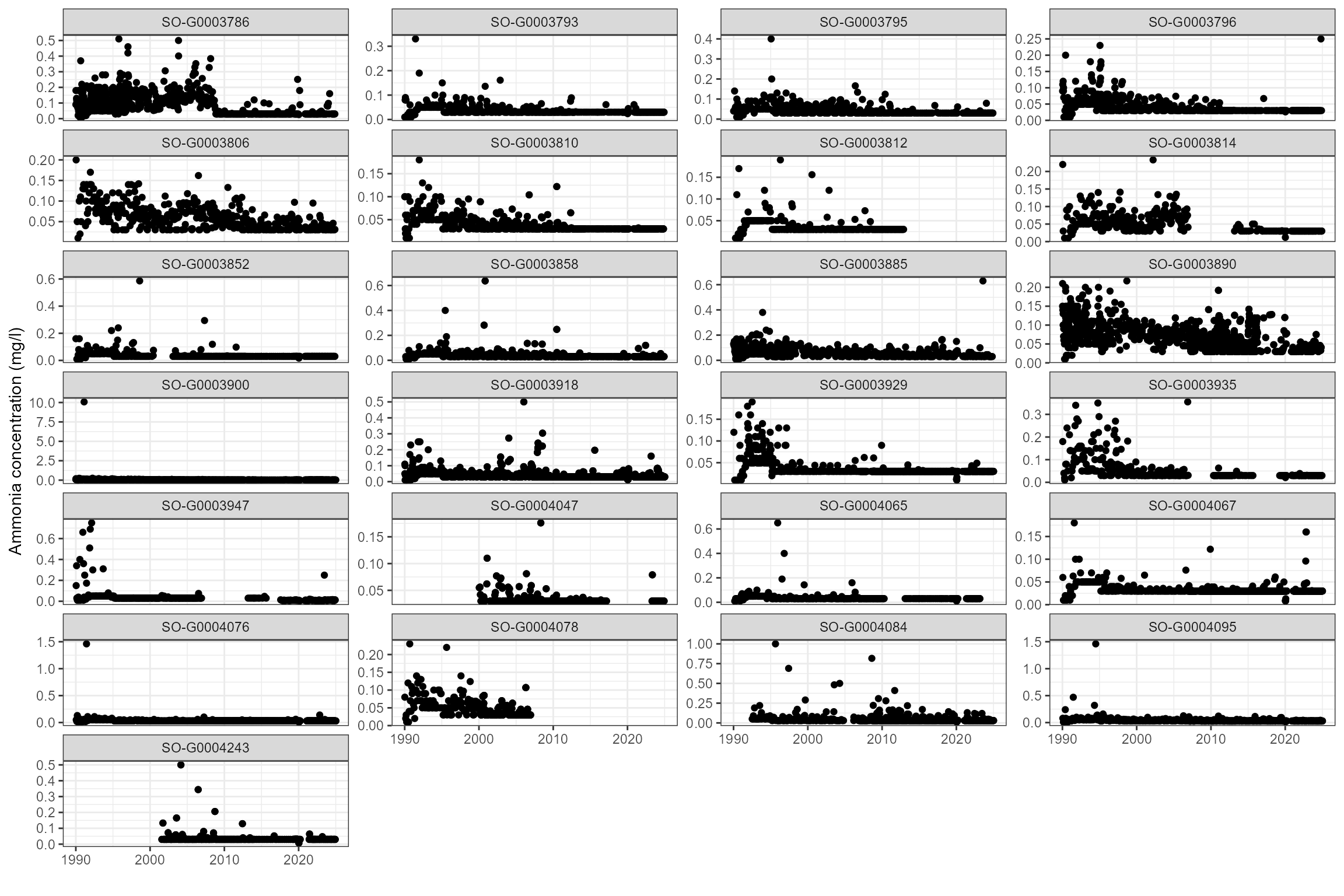
cs1_wq_data %>%
dplyr::filter(det_label == "Orthophospht") %>%
ggplot(aes(x = date, y = result)) +
geom_point() +
ylab("Orthophosphate concentration (mg/l)") +
xlab("") +
facet_wrap(~ wq_site_id, scales = "free_y", ncol = 4)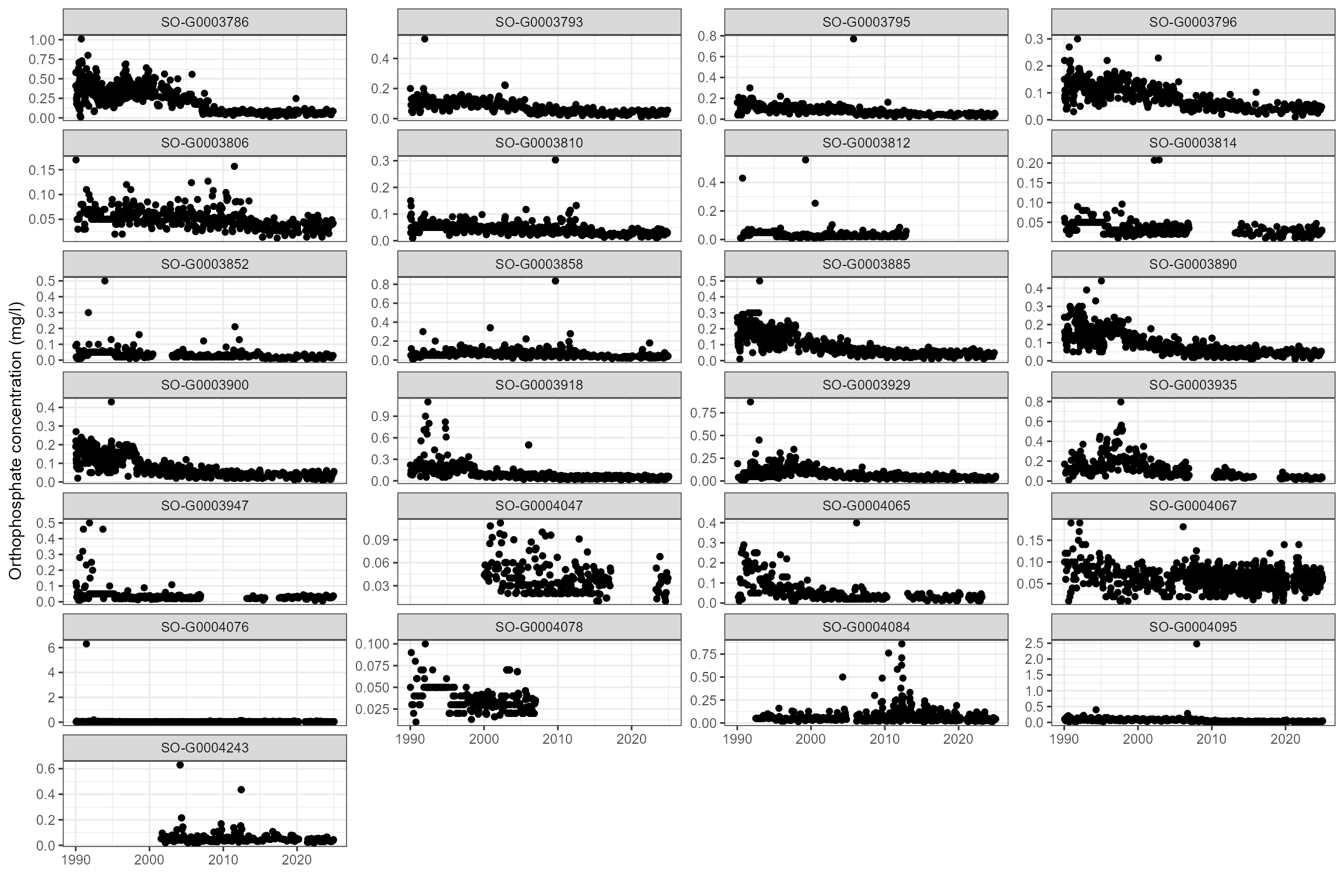
Following the Water Framework Directive (WFD) approach to classification, we choose to calculate the 90th percentile ammonia concentration and mean orthophosphate concentration for a rolling three year period at each site.
# Calculate rolling 3-year summary statistics, by site and id.
cs1_wq_summary <- expand.grid(year = seq(from = 1995, to = 2019),
wq_site_id = unique(cs1_metadata$wq_site_id))
for(i in 1:dim(cs1_wq_summary)[1]){
# Filter down to rolling three year window
temp <- cs1_wq_data %>%
dplyr::filter(year <= cs1_wq_summary$year[i] & year >= cs1_wq_summary$year[i]-2)
# Calculate mean orthophsophate
cs1_wq_summary$mean_p[i] <- mean(temp$result[temp$det_label == "Orthophospht" &
temp$wq_site_id == cs1_wq_summary$wq_site_id[i]], na.rm = TRUE)
# Calculate 90th percentile ammonia
cs1_wq_summary$ammonium_90[i] <- quantile(temp$result[temp$det_label == "Ammonia(N)" &
temp$wq_site_id == cs1_wq_summary$wq_site_id[i]], 0.90, na.rm=TRUE)
rm(temp)
}
# Infill NAs using values for neighbouring years
cs1_wq_summary <- cs1_wq_summary %>%
dplyr::group_by(wq_site_id) %>%
tidyr::fill(mean_p, .direction = "downup") %>%
tidyr::fill(ammonium_90, .direction = "downup") %>%
dplyr::ungroup()These are the resulting rolling three-year summary statistics for each water quality site:
# Plot calculated summary statistics
cs1_wq_summary %>%
ggplot(aes(x = year, y = mean_p)) +
geom_point() +
facet_wrap(~wq_site_id)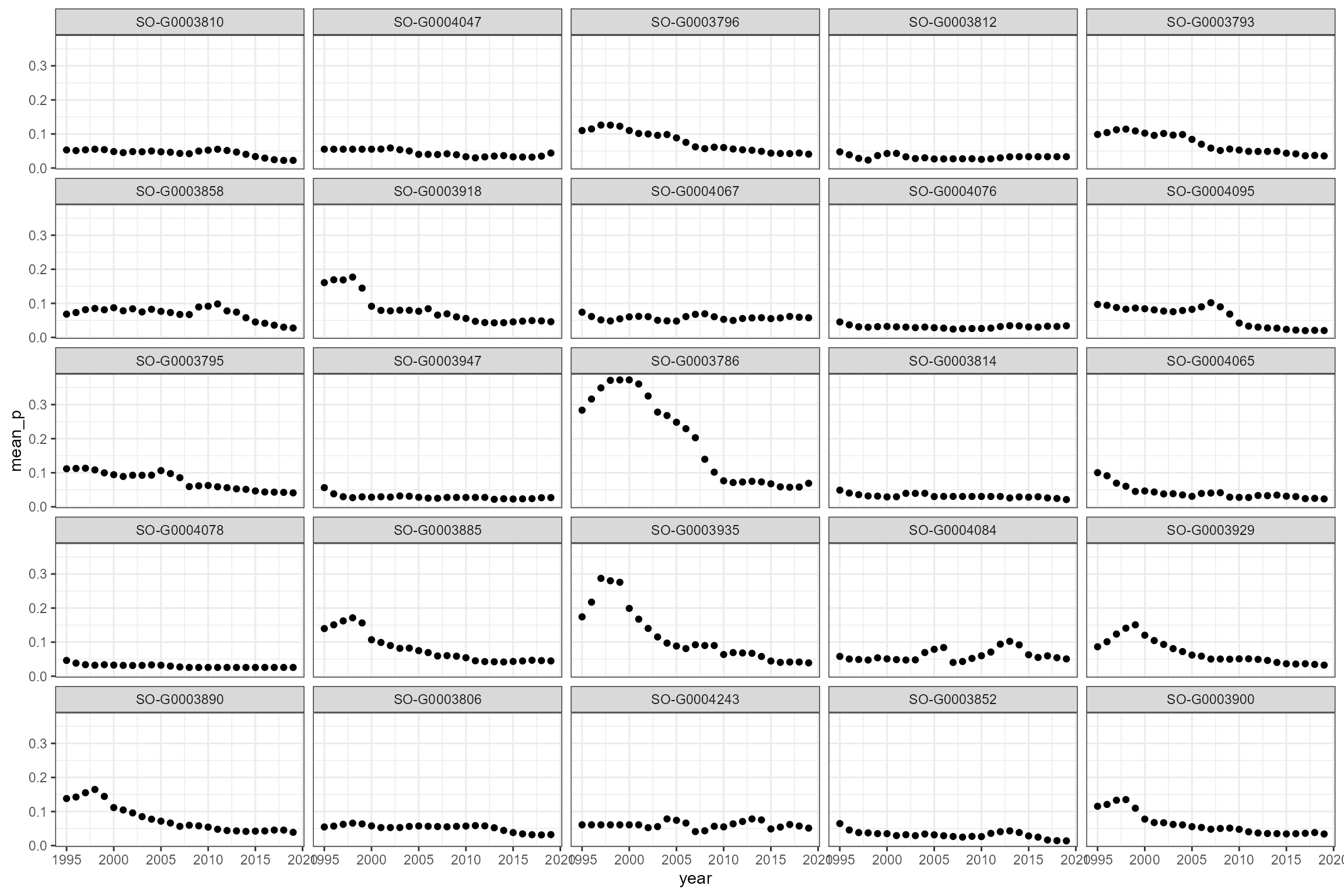
cs1_wq_summary %>%
ggplot(aes(x = year, y = ammonium_90)) +
geom_point() +
facet_wrap(~wq_site_id)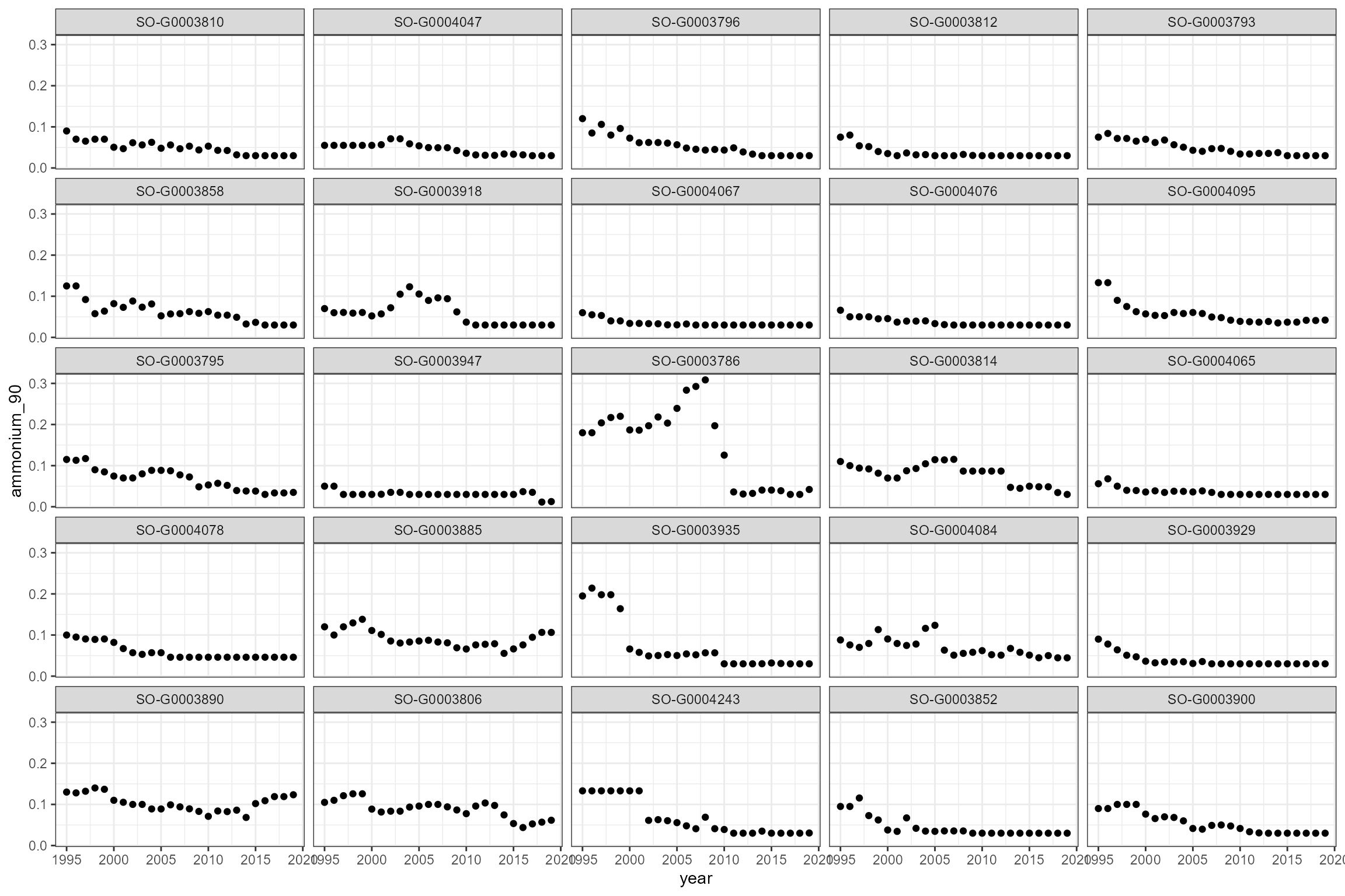
# check distributions and correlations
cs1_wq_summary %>%
dplyr::select(mean_p, ammonium_90) %>%
scatterPlotMatrix(distribType = 1, corrPlotType = "Text", width = 600, height = 600)Ammonia and orthophosphate are strongly correlated (r = 0.70), so we choose to use just one (ammonia) to use as a predictor variable in our model. We choose ammonia based on scientific literature showing that ammonia is more likely to have a direct effect on macroinvertebrate community, whereas orthophosphate has an indirect effect by impacting food and habitat. The ammonia variable therefore provides a indicator of general water quality.
Flow data
Modelled time series of historical and naturalised flows on a 7-daily time step were exported from the Test and Itchen (T&I) groundwater model for the period 1965-2017. (Estimated flows under Recent Actual and Fully Licenced conditions were also available but not used). Note that there are just 31 unique flow sites (stream cells) linked to the 33 macroinvertebrate sites. The data, stored as an RDS file, were then manually imported into R:
Import raw flow data
# Read in flow data in long format (four flow scenarios stacked)
cs1_flowraw_long <- readRDS("Data/caseStudy1/cs1_flows.rds") %>%
# Rename to facilitate later data joining
dplyr::rename(flow_site_id = ReachID) %>%
# Add year column
dplyr::mutate(Year = lubridate::year(Date)) %>%
# Format site as factor
dplyr::mutate(flow_site_id = factor(flow_site_id)) %>%
# Filter to start a few years before biology sample data
dplyr::filter(Year >= 1990)
# Convert to wide format (one column for each flow scenario)
cs1_flowraw_wide <- cs1_flowraw_long %>%
tidyr::pivot_wider(names_from = Scenario, values_from = Flow)Compare the long and wide format of the flow data:
## # A tibble: 6 × 5
## flow_site_id Date Flow Scenario Year
## <fct> <date> <dbl> <chr> <dbl>
## 1 TI12911 1990-01-02 25670. Historical 1990
## 2 TI13105 1990-01-02 20737. Historical 1990
## 3 TI13525 1990-01-02 80659. Historical 1990
## 4 TI13598 1990-01-02 53227. Historical 1990
## 5 TI13963 1990-01-02 64400. Historical 1990
## 6 TI14055 1990-01-02 56400. Historical 1990## # A tibble: 6 × 7
## flow_site_id Date Year Historical Naturalised RecentActual
## <fct> <date> <dbl> <dbl> <dbl> <dbl>
## 1 TI12911 1990-01-02 1990 25670. 25889. 25592.
## 2 TI13105 1990-01-02 1990 20737. 24821. 20843.
## 3 TI13525 1990-01-02 1990 80659. 78787. 82152.
## 4 TI13598 1990-01-02 1990 53227. 56551. 56563.
## 5 TI13963 1990-01-02 1990 64400. 66675. 66646.
## 6 TI14055 1990-01-02 1990 56400. 61591. 60819.
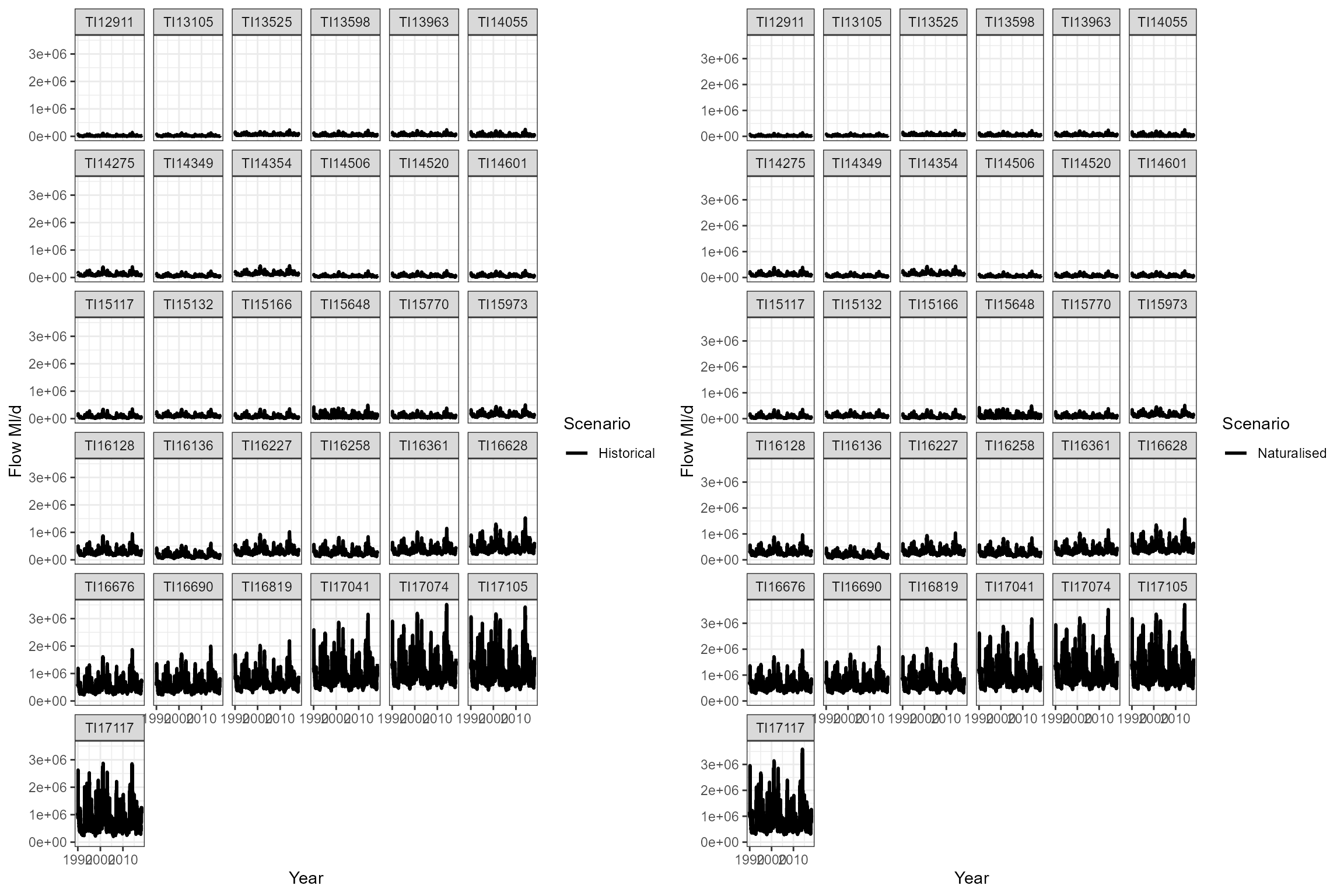
## # ℹ 1 more variable: FullyLicensed <dbl>Raw data plots
The following plots show, for each groundwater model area in turn, the modelled historical and modelled naturalised flows at each location.
Flow statistics
The flow data were processed to calculate (i) the degree of long-term flow alteration, and (ii) a time-varying metric of flow history, designed to capture the effect of inter-annual variation in flow.
Flow alteration metric
To quantify the degree of abstraction pressure at each site, the historical Q95 was calculated and expressed as a ratio of the naturalised Q95 to yield a Q95 Residual Flow Ratio (RFR) variable. A ratio of 1 indicates that were flows are not influenced (i.e. at natural); ratios <1 indicate a progressively greater degree of abstraction pressure (i.e. flow reduction), and ratios >1 indicates that flows are higher than natural (i.e. the watercourse is discharge-rich).
We first calculate a time series of annual RFRs for each site, to check whether the degree of flow alteration has changed over time:
# Calculate and plot annual flow alteration statistics for each site
cs1_flowraw_wide %>%
group_by(flow_site_id, Year) %>%
dplyr::summarise(LTQ95hist = quantile(Historical, 0.05, na.rm=TRUE),
LTQ95nat = quantile(Naturalised, 0.05, na.rm=TRUE)) %>%
mutate(LTQ95RFR = LTQ95hist / LTQ95nat) %>%
ggplot(aes(x = Year, y = LTQ95RFR)) +
geom_line() +
facet_wrap(~flow_site_id, nrow = 4) +
labs(x = "Year", y = "Residual Flow Ratio at Q95") +
theme_bw()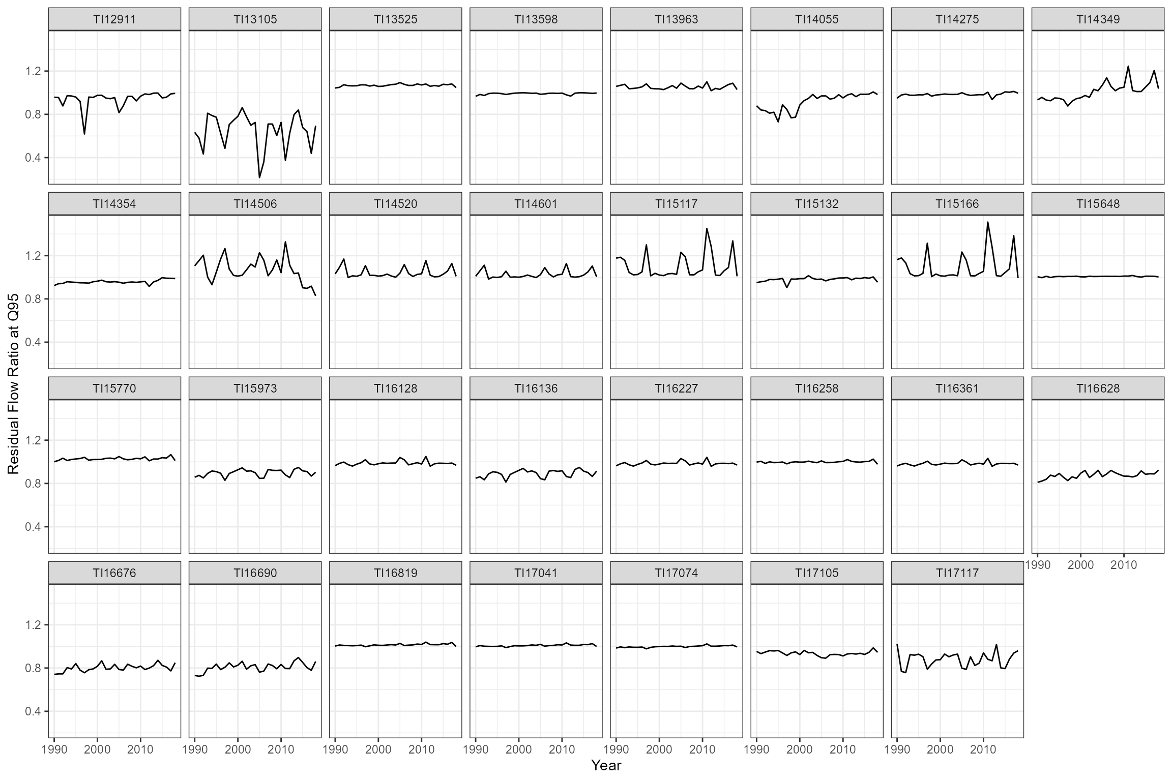
There is inter-annual variability in the degree of flow alteration at
some sites, but no evidence of long-term trends that might indicate
systematic changes in abstraction pressure. We therefore choose to
calculate a long-term RFR for each site (termed LTQ95RFR)
and use this in our model as a measure of flow alteration.
Flow history metric
The calc_flowstats function takes a time series of a
measured or modelled flows and uses a user-defined moving window to
calculate a suite of time-varying flow statistics for one or more sites.
Below, calc_flowstats is used to calculate the Q95 for a
moving 12 month window. The Q95 values are then standardised to make
them dimensionless and comparable among sites.
# Set any negative flow values to NA's
cs1_flowraw_wide$Historical[cs1_flowraw_wide$Historical <= 0] <- NA
# Use calc_flowstats() function to calculate Q95z (this may take a few minutes)
cs1_flowstats <- hetoolkit::calc_flowstats(data = cs1_flowraw_wide,
site_col= "flow_site_id",
date_col= "Date",
flow_col= "Historical",
imputed_col= NULL,
win_start = "1990-01-01",
win_width = "1 year",
win_step = "1 month",
date_range = NULL)
# Extract data frame of time-varying flow statistics, and select only essential columns
cs1_flowstats1 <- cs1_flowstats[[1]] %>%
dplyr::select("flow_site_id", "win_no", "start_date", "end_date", "Q95z")
# Remove rows where Q95z is NA (2018 onwards)
cs1_flowstats1 <- cs1_flowstats1[complete.cases(cs1_flowstats1$Q95z), ]
# Extract long-term flow statistics
cs1_flowstats_2 <- cs1_flowstats[[2]]Visualise the standardised time-varying Q95 statistics:
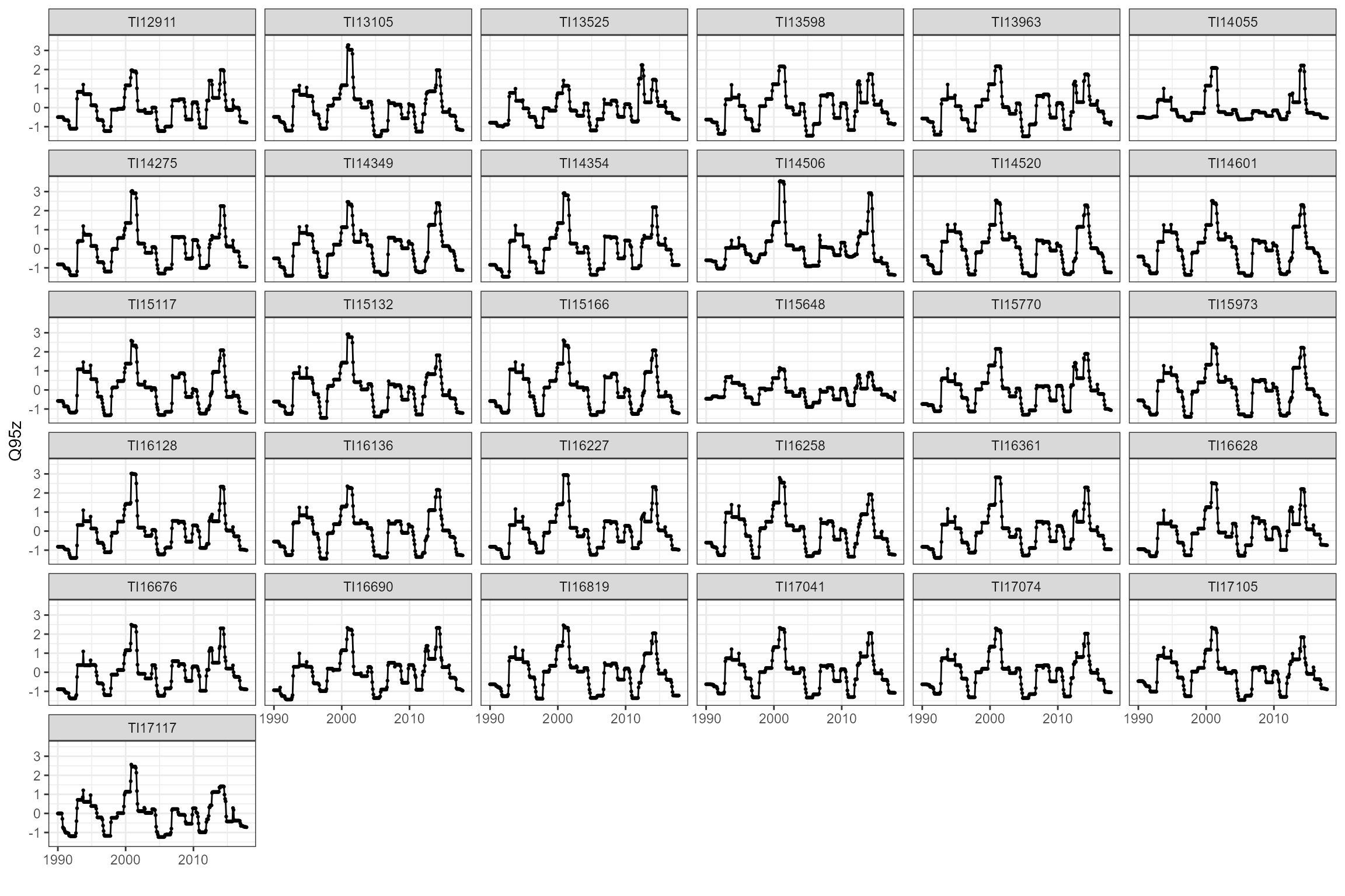
Join hydrological and ecological data
The join_he function links biology data with
time-varying flow statistics for one or more antecedent (lagged) time
periods (as calculated by the calc_flowstats function) to
create a combined dataset for hydro-ecology modelling. Here we use
method = "A" and lags = c(0,12) to get the
flow statistics for the immediately preceding 12 month period, and the
12 month period before that. For example, a macroinvertebrate sample
collected in April 2015 will be joined with flow statistics for the
periods April 2014-March 2015 (lag 0) and April 2013-March 2014 (lag
12).
# Join flow statistics to biology data to create a dataset for model calibration
cs1_he1 <- hetoolkit::join_he(biol_data = cs1_biol_all,
flow_stats = cs1_flowstats1,
mapping = cs1_metadata,
lags = c(0,12),
method = "A",
join_type = "add_flows") %>%
# Manually join the long-term flow alteration statistics, RHS metrics and
# water quality statistics for each site
dplyr::left_join(cs1_rfr, by = "flow_site_id") %>%
dplyr::left_join(cs1_rhs_data, by = "rhs_survey_id") %>%
dplyr::left_join(cs1_wq_summary, by = c("wq_site_id", "Year" = "year"))
# Separately, join biology data to flow statistics to create a dataset for data visualisation
# (this feeds into the plot_rngflows function)
cs1_he2 <- hetoolkit::join_he(biol_data = cs1_biol_all,
flow_stats = cs1_flowstats1,
mapping = cs1_metadata,
lags = c(0,12),
method = "A",
join_type = "add_biol")View the first dataset created using
join_type = "add_flows":
And now the second dataset created using
join_type = "add_biol":
Modelling
Assess coverage of historical flow conditions
The plot_rngflows function generates a scatterplot for
two flow variables and overlays two convex hulls: one showing the full
range of flow conditions experienced historically, and a second convex
hull showing the range of flow conditions with associated biology
samples. This visualization helps identify to what extent the available
biology data span the full range of flow conditions experienced
historically.
In the following example, we plot the Q95z flow statistics in each of the previous two years. The first plot shows the data for all sites; the second plot is faceted to show the data separately for each site individually. In this dataset, the orange polygon almost completely fills the grey polygon, indicating that the biology samples provide excellent coverage of historical flow conditions.
hetoolkit::plot_rngflows(data = cs1_he2,
flow_stats = c("Q95z_lag0","Q95z_lag12"),
biol_metric = "LIFE_F_OE")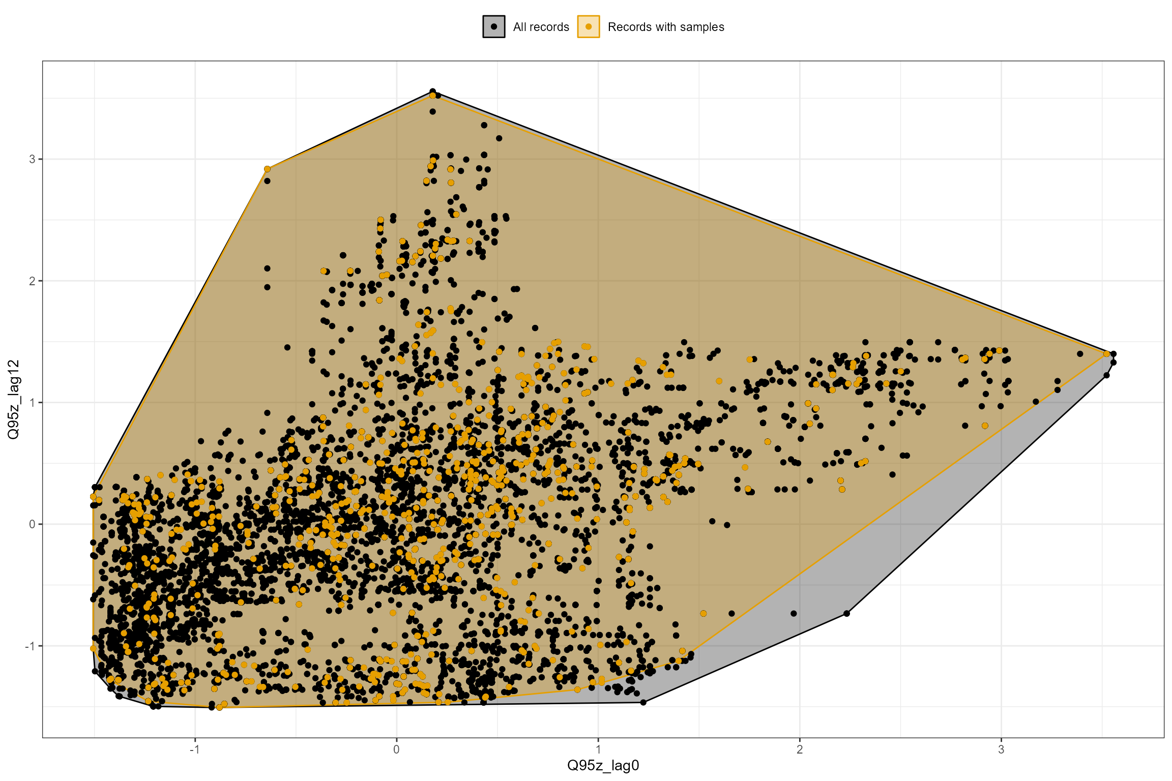
hetoolkit::plot_rngflows(data = cs1_he2,
flow_stats = c("Q95z_lag0", "Q95z_lag12"),
biol_metric = "LIFE_F_OE",
wrap_by = "biol_site_id",
label = "Year")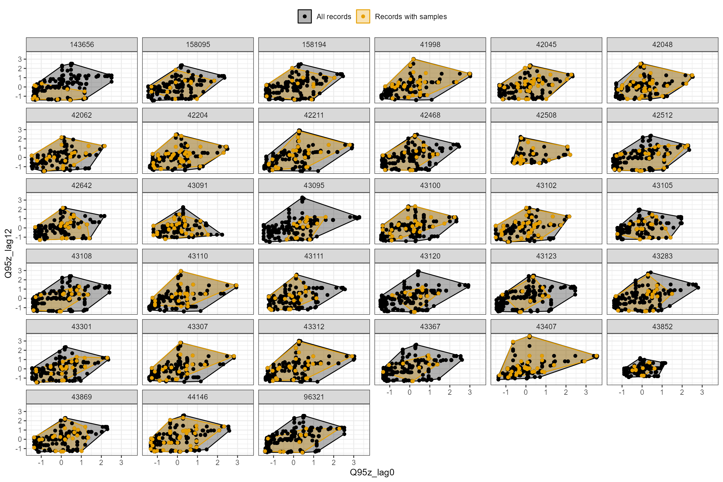
Data preparation
We use pairwise plots to identify highly correlated variables (that might need to be excluded as candidate predictor variables), skewed variables (e.g. ammonium_90, that might benefit from transformation), and gross outliers (none found).
# produce pairs plot
cs1_he1 %>%
dplyr::select(LTQ95RFR, ammonium_90, Q95z_lag0, Q95z_lag12, HMSRBB, LIFE_F_OE) %>%
scatterPlotMatrix(distribType = 1, corrPlotType = "Text", width = 800, height = 600)We then transform, scale and filter our data to produce a final dataset ready for modelling:
# prepare data
cs1_he1 <- cs1_he1 %>%
# make season a factor
dplyr::mutate(Season = as.factor(Season)) %>%
# center year variable (which aids model convergence)
dplyr::mutate(Year_2005 = Year - 2005) %>%
# log-transform ammonia
dplyr::mutate(log10_ammonium_90 = log10(ammonium_90)) %>%
# remove records with NAs for response or predictor variables
dplyr::filter(is.na(log10_ammonium_90) == FALSE) %>%
# re-scale HMSRBB scores to avoid scaling issues in model
dplyr::mutate(HMSRBB = HMSRBB/100)
# check the number of rows and columns in the final dataset
dim(cs1_he1)## [1] 746 25Model calibration
Using a linear mixed-effects model fitted via the lmer()
function, we model spatial variation in LIFE O:E as a function of
long-term flow alteration (LTQ95RFR) and the extent of bed
and bank re-sectioning (HMSRBB), and temporal variation in
LIFE O:E as a function of flow history over the preceding 1-12 months
(Q95z_lag0) and over the preceding 13-24 months
(Q95z_lag12). Interactions with Season were
included to test the hypothesis that LIFE O:E ratios in spring and
autumn respond differently to flow history. In addition,
log10_ammonium_90 was included as a main effect to
represent general water quality over the previous three years. (We used
a 3 year moving window to mirror the WFD rolling classification process,
however further analysis could be undertaken to compare how sensitive
results are to differing window widths.) Year_2005 (year,
centered so that 2005 = 0) was also included to account for long-term
trends unrelated to general water quality (insofar as these are
represented by the log10_ammonium_90 variable).
Site (biol_site_id) was included as a random intercept
to measure unexplained spatial variation in LIFE O:E and
Year_2005 had a random slope to account for site-specific
trends. (There were insufficient data to fit multiple random slopes, and
exploratory analysis suggested that Year was a key variable).
First we fit a full model containing all of these terms. Note the use
of the lmerTest package, which provides
approximate p-values for fixed effects in
summary():
# fit full model
cs1_mod1 <- lmerTest::lmer(LIFE_F_OE ~
Season +
Year_2005 +
HMSRBB +
LTQ95RFR +
Q95z_lag0 * Season +
Q95z_lag12 * Season +
log10_ammonium_90 +
(Year_2005 | biol_site_id),
data = cs1_he1,
REML = FALSE,
control = lmerControl(optimizer="bobyqa", optCtrl = list(maxfun = 10000)))
summary(cs1_mod1)## Linear mixed model fit by maximum likelihood . t-tests use Satterthwaite's
## method [lmerModLmerTest]
## Formula: LIFE_F_OE ~ Season + Year_2005 + HMSRBB + LTQ95RFR + Q95z_lag0 *
## Season + Q95z_lag12 * Season + log10_ammonium_90 + (Year_2005 |
## biol_site_id)
## Data: cs1_he1
## Control: lmerControl(optimizer = "bobyqa", optCtrl = list(maxfun = 10000))
##
## AIC BIC logLik -2*log(L) df.resid
## -2766.7 -2702.1 1397.4 -2794.7 732
##
## Scaled residuals:
## Min 1Q Median 3Q Max
## -2.6110 -0.5881 -0.0014 0.5827 10.1729
##
## Random effects:
## Groups Name Variance Std.Dev. Corr
## biol_site_id (Intercept) 8.756e-04 0.029590
## Year_2005 1.331e-06 0.001154 -0.23
## Residual 1.193e-03 0.034538
## Number of obs: 746, groups: biol_site_id, 33
##
## Fixed effects:
## Estimate Std. Error df t value Pr(>|t|)
## (Intercept) 1.021e+00 4.674e-02 3.985e+01 21.839 < 2e-16 ***
## SeasonSpring -6.091e-03 2.587e-03 6.874e+02 -2.354 0.018837 *
## Year_2005 2.427e-03 4.216e-04 7.774e+01 5.757 1.63e-07 ***
## HMSRBB -2.712e-04 8.321e-04 3.222e+01 -0.326 0.746593
## LTQ95RFR 9.524e-03 4.530e-02 3.198e+01 0.210 0.834826
## Q95z_lag0 2.382e-02 2.637e-03 6.999e+02 9.033 < 2e-16 ***
## Q95z_lag12 -3.215e-03 2.433e-03 6.982e+02 -1.322 0.186747
## log10_ammonium_90 -2.176e-02 1.401e-02 4.615e+02 -1.553 0.121143
## SeasonSpring:Q95z_lag0 -1.106e-02 3.332e-03 6.932e+02 -3.319 0.000951 ***
## SeasonSpring:Q95z_lag12 9.095e-03 3.131e-03 6.920e+02 2.905 0.003788 **
## ---
## Signif. codes: 0 '***' 0.001 '**' 0.01 '*' 0.05 '.' 0.1 ' ' 1
##
## Correlation of Fixed Effects:
## (Intr) SsnSpr Y_2005 HMSRBB LTQ95R Q95z_0 Q95_12 l10__9 SS:Q95_0
## SeasonSprng -0.029
## Year_2005 0.235 -0.004
## HMSRBB 0.014 -0.005 -0.026
## LTQ95RFR -0.918 0.005 -0.002 -0.095
## Q95z_lag0 -0.002 0.089 0.023 0.003 0.015
## Q95z_lag12 0.014 0.004 0.081 0.000 -0.007 -0.383
## lg10_mmn_90 0.361 0.005 0.647 -0.060 0.016 0.048 0.017
## SsnSp:Q95_0 0.012 -0.128 0.020 -0.004 -0.011 -0.783 0.309 -0.009
## SsnS:Q95_12 -0.005 -0.075 -0.054 0.001 0.004 0.297 -0.771 -0.004 -0.368The p-values from summary() are only approximate and
cannot be relied upon to guide model selection. Nonetheless, some of the
terms appear to be non-significant, suggesting that some model
simplification may be beneficial.
Here we use the HE Toolkit’s model_logocv function to
perform cross validation and guide a backwards elimination process with
the goal of identifying a more parsimonious model. Cross validation -
testing how well the model is able to predict LIFE O:E at each site in
turn when that site is dropped from the calibration dataset - provides a
robust measure of the model’s predictive performance (quantified as the
Root Mean Square Error, or RMSE), and can be used to identify and
eliminate unimportant variables. In this case study, the primary focus
is on assessing the influence of flow alteration on spatial patterns in
LIFE O:E ratios and so we choose to use the model_logocv
function, which puts more emphasis on the model’s ability to explain
spatial variation, over the model_cv function, which puts
more emphasis on temporal variation.
Note that to use the model_logocv function, models need
to be fitted using the lme4 (not lmerTest)
package.
# fit full model using lme4 package
cs1_mod1 <- lme4::lmer(LIFE_F_OE ~
Season +
Year_2005 +
HMSRBB +
LTQ95RFR +
Q95z_lag0 * Season +
Q95z_lag12 * Season +
log10_ammonium_90 +
(Year_2005 | biol_site_id),
data = cs1_he1,
REML = FALSE,
control = lmerControl(optimizer="bobyqa", optCtrl = list(maxfun = 10000)))
summary(cs1_mod1)
# calculate RMSE for the full model
cs1_mod1_logocv <- hetoolkit::model_logocv(model = cs1_mod1,
data = cs1_he1,
group = "biol_site_id",
control = lmerControl(optimizer="bobyqa",
optCtrl = list(maxfun = 10000)))
# get the RMSE (smaller values are better)
cs1_mod1_logocv[[1]]Model simplification is conducted in a stepwise manner, with one term being eliminated at a time, until no further improvement in the RMSE can be achieved. Following this process (not shown for brevity), the final model is:
# fit final model
cs1_mod2 <- lme4::lmer(LIFE_F_OE ~
Season +
Year_2005 +
# HMSRBB +
# LTQ95RFR +
Q95z_lag0 * Season +
Q95z_lag12 * Season +
# log10_ammonium_90 +
(1 | biol_site_id),
data = cs1_he1,
REML = FALSE,
control = lmerControl(optimizer="bobyqa", optCtrl = list(maxfun = 10000)))
cs1_mod2_logocv <- hetoolkit::model_logocv(model = cs1_mod2,
data = cs1_he1,
group = "biol_site_id",
control = lmerControl(optimizer="bobyqa", optCtrl = list(maxfun = 10000)))Comparing the RMSE values for the full and final models:
# mod2 has the smaller RMSE, so is the preferred model
cs1_mod1_logocv[[1]]## [1] 0.04923244
cs1_mod2_logocv[[1]]## [1] 0.04638482Model interpretation
## Linear mixed model fit by maximum likelihood ['lmerMod']
## Formula: LIFE_F_OE ~ Season + Year_2005 + Q95z_lag0 * Season + Q95z_lag12 *
## Season + (1 | biol_site_id)
## Data: cs1_he1
## Control: lmerControl(optimizer = "bobyqa", optCtrl = list(maxfun = 10000))
##
## AIC BIC logLik -2*log(L) df.resid
## -2763.2 -2721.6 1390.6 -2781.2 737
##
## Scaled residuals:
## Min 1Q Median 3Q Max
## -2.5713 -0.6219 0.0075 0.5863 9.7771
##
## Random effects:
## Groups Name Variance Std.Dev.
## biol_site_id (Intercept) 0.0008666 0.02944
## Residual 0.0012469 0.03531
## Number of obs: 746, groups: biol_site_id, 33
##
## Fixed effects:
## Estimate Std. Error t value
## (Intercept) 1.0564938 0.0054766 192.910
## SeasonSpring -0.0061608 0.0026441 -2.330
## Year_2005 0.0028753 0.0002262 12.713
## Q95z_lag0 0.0239843 0.0026830 8.939
## Q95z_lag12 -0.0029568 0.0024789 -1.193
## SeasonSpring:Q95z_lag0 -0.0109882 0.0034007 -3.231
## SeasonSpring:Q95z_lag12 0.0088905 0.0031962 2.782
##
## Correlation of Fixed Effects:
## (Intr) SsnSpr Y_2005 Q95z_0 Q95_12 SS:Q95_0
## SeasonSprng -0.235
## Year_2005 0.028 -0.011
## Q95z_lag0 -0.049 0.088 -0.008
## Q95z_lag12 0.005 0.004 0.111 -0.385
## SsnSp:Q95_0 0.039 -0.128 0.040 -0.785 0.308
## SsnS:Q95_12 -0.001 -0.075 -0.083 0.298 -0.772 -0.367The preferred model with the lowest RMSE score (model 2) included the
fixed predictors Season, Year_2005, and
Q95z_lag0 and Q95z_lag12 interacting with
Season, while the random effects included an intercept
varying by site. Thus, there was no evidence that LIFE O:E was
influenced by water quality (log10_ammonium_90), long-term
flow alteration (LTQ95RFR), or the extent of bed and bank
re-sectioning (HMSRBB). In the case of water quality and
flow alteration, this may be because the 33 sites spanned only a narrow
pressure gradient; ammonia concentrations were mostly at High or Good
status, and at only one site was the long-term Q95 reduced by more than
25%.
On average, LIFE O:E was fractionally lower in spring than autumn, and there was an increasing long-term trend across all sites of ca 0.0029 per year (equating to an increase of nearly 0.07 over the 24 year time period of the data). After accounting for these effects, LIFE O:E was positively associated with Q95z_lag0 (low flows in the preceding 12 month period), and this relationship was stronger in autumn than in spring. By contrast, LIFE O:E was only weakly associated with Q95z_lag12 (low flows in the year before last), showing a small negative effect in autumn and a small positive effect in spring.
The random variance of the intercept was estimated to be 0.0009, meaning that the unexplained spatial variation among the sites was in the range of +/- 0.05 (see caterpillar plot below). The residual variance was larger (0.0012), indicating slightly more temporal variation than spatial variation left unexplained by the model.
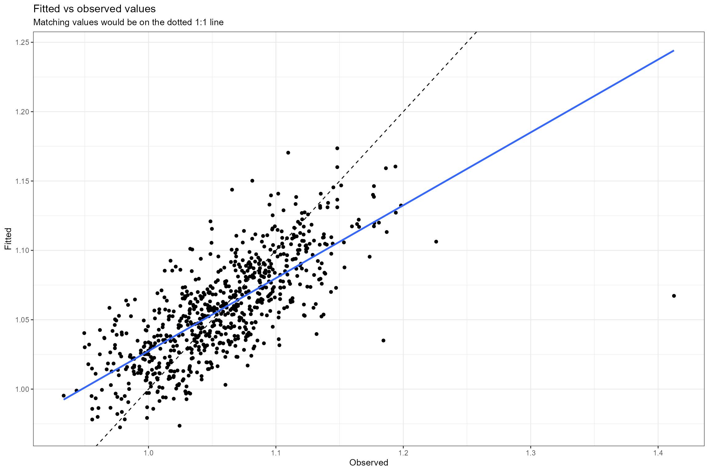
Model diagnostics
The diag_lmer function produces a variety of diagnostic
plots for a mixed-effects regression (lmer) model. Below we create model
diagnostic plots for the final model (cs1_mod2).
# generate diagnostic plots
cs1_diag_plots <- hetoolkit::diag_lmer(
model = cs1_mod2,
data = cs1_he1,
facet_by = NULL)These include:
- Fitted vs observed values. This plot shows the relationship between the fitted (predicted) and observed (true) values of the response variable. If the model fits the data well, the points should be clustered around the diagonal 1:1 line, which represents a perfect fit (fitted = observed). Here we can see the model provides a reasonably good fit to the data, but with a slight tendency to under-predict high LIFE O:E ratios and over-predict low LIFE O:E ratios (which is very common in regression modelling).
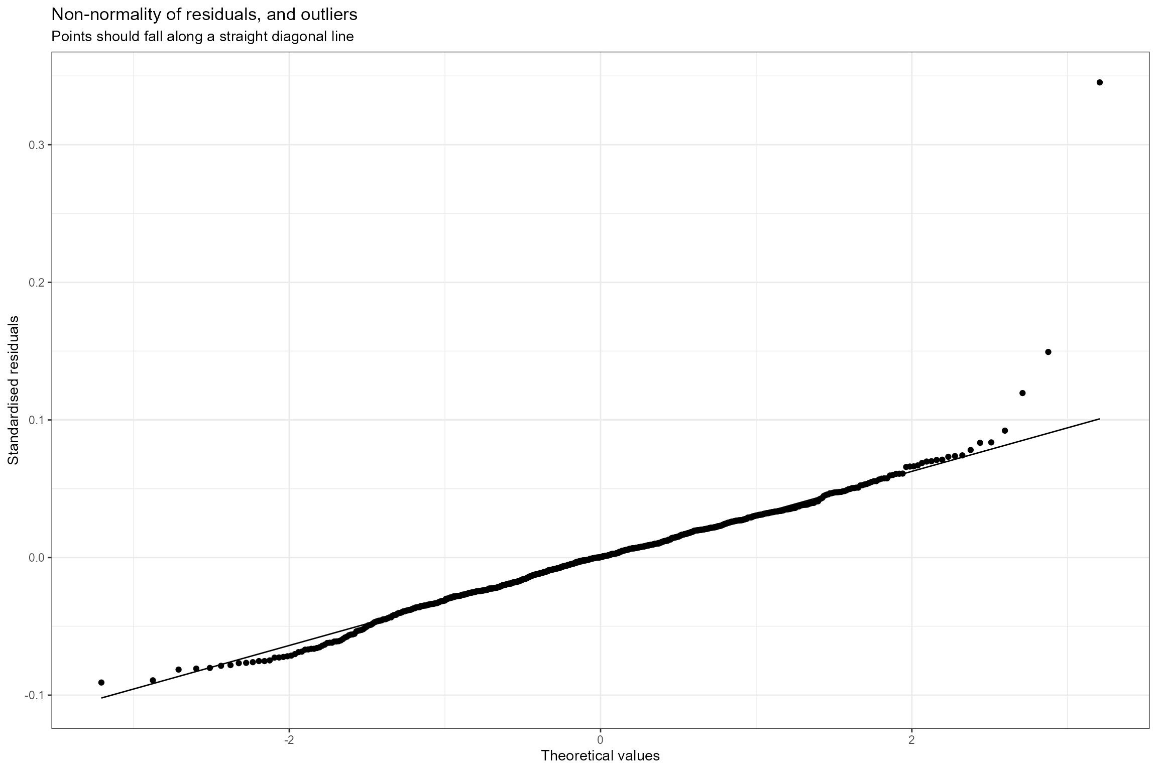
- Normal probability plot. This is a graphical technique for verifying the assumption of a Normally-distributed error structure. The model residuals are plotted against a theoretical Normal distribution in such a way that the points should form an approximate straight line. Here we can see that the residuals conform very closely to a Normal distribution, with just three data points having unusually large positive residuals.
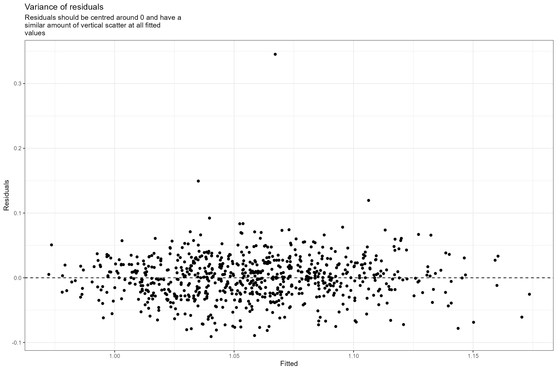
- Residuals vs fitted values. This plot checks the assumption of homogeneous variances, which states that the error variance should be constant regardless of what value the response takes. Here we can see that the residuals have a similar amount of vertical scatter at all fitted values of the response, so this assumption is verified.
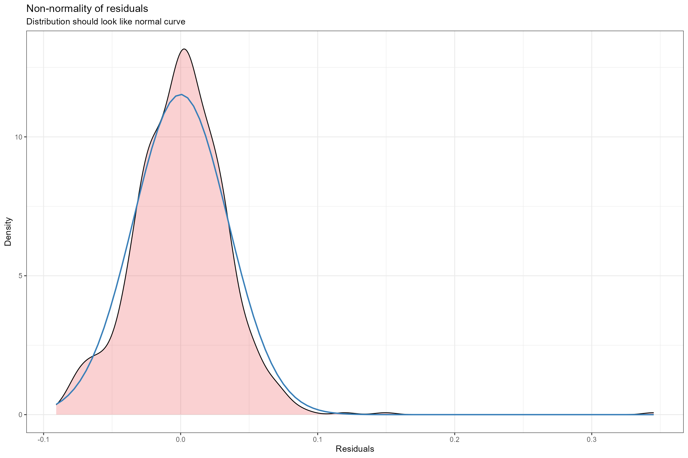
- Histogram of residuals. This is an alternative to plot 2 for verifying the assumption of Normally-distributed errors. Here we can see that the probability distribution of the model residuals (shown by the pink shaded area) is very similar to a perfect Normal distribution (shown by the blue line).
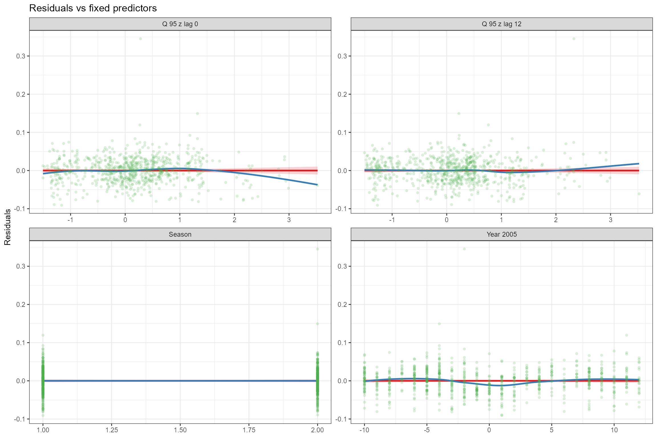
- Residuals vs fixed predictors. To verify the assumption of linearity, the model’s residuals are plotted against each of the fixed predictors in turn. If the relationship between the response and each predictor is truly linear, then there should be no trend in the residuals. We can see that the linear (red) line fitted to the residuals is horizontal, indicating that that the strength of the linear effects has not been over- or under-estimated. And the loess-smoothed (blue) line is also close to horizontal; there is a small departure from linearity at high Q95z values but this is driven by a small number of data points so, overall, the modelled relationships are close to linear.
Other useful diagnostic plots for lmer models
include:
- Caterpillar plots, for visualising the random effects for each site. Our final model only has a random intercept, so the plot shows the estimated random effect (expressed as a deviation from the global intercept) for each site (biol_site_id). Sites coloured blue are those where, all else being equal, the mean LIFE O:E ratio is higher than average, and red sites have lower-than-average LIFE O:E ratios. This confirms that there is reasonably large (+/- 0.05) variation in LIFE O:E ratios from site to site that cannot be explained by the other, fixed effects in the model.
sjPlot::plot_model(model = cs1_mod2,
type = "re",
facet.grid = FALSE,
free.scale = FALSE,
title = NULL,
vline.color = "darkgrey") +
ylim(-0.1,0.1)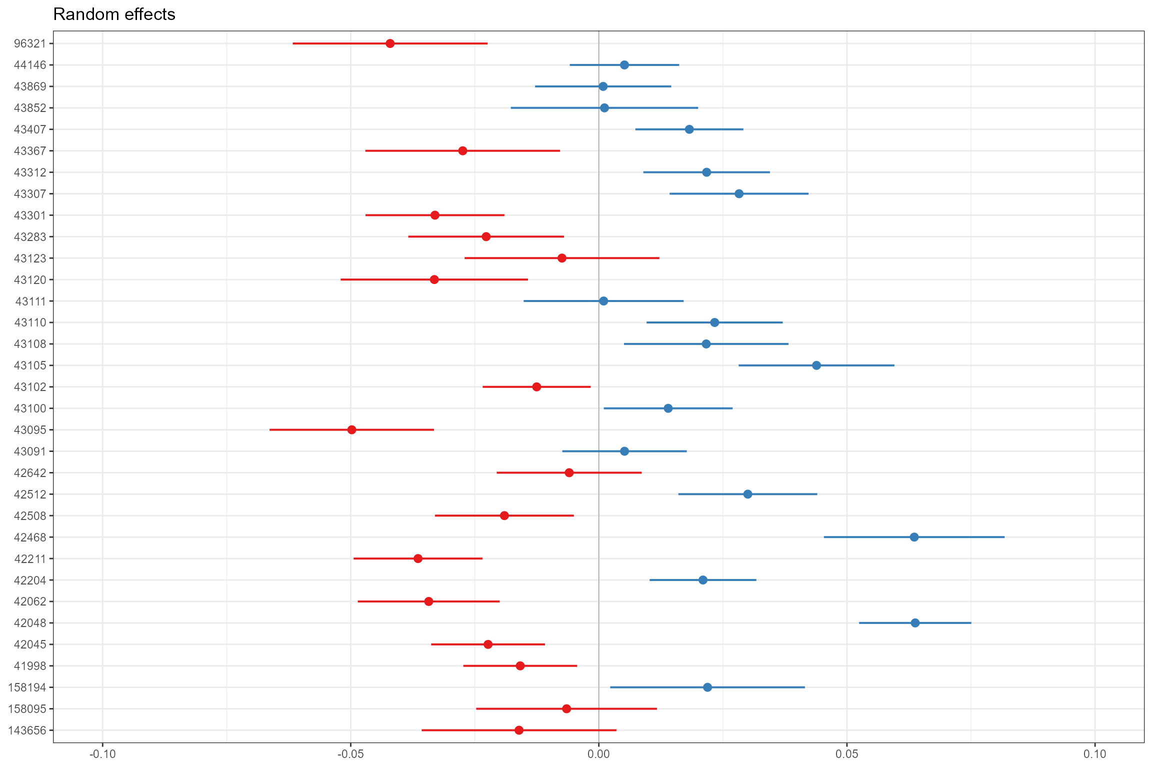
- Partial effects plots, for visualising the modelled effect of each fixed predictor variable in turn when other continuous predictors are held constant at their mean values and factors are fixed at their reference level (i.e. autumn for Season). This confirms the strong positive association of LIFE O:E ratios with year and Q95z in the previous 12 months.
sjPlot::plot_model(model = cs1_mod2,
type = "pred",
pred.type = "fe",
facet.grid = TRUE,
scales = "fixed", terms = "Season")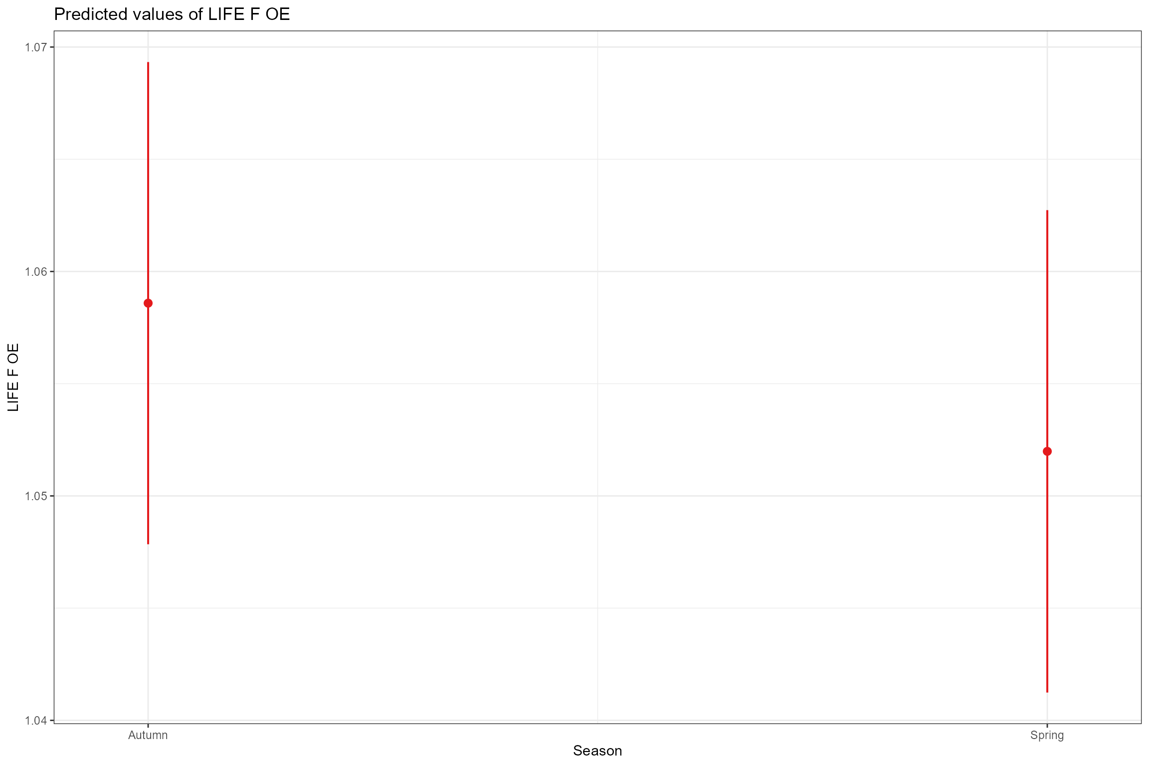
sjPlot::plot_model(model = cs1_mod2,
type = "pred",
pred.type = "fe",
facet.grid = TRUE,
scales = "fixed", terms = "Year_2005")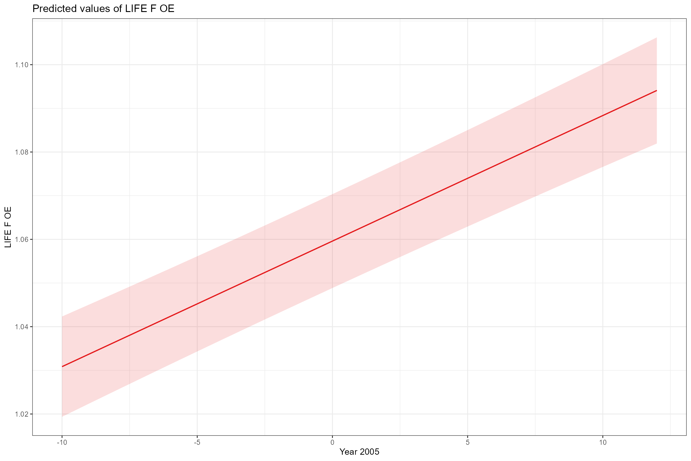
sjPlot::plot_model(model = cs1_mod2,
type = "pred",
pred.type = "fe",
facet.grid = TRUE,
scales = "fixed", terms = "Q95z_lag0")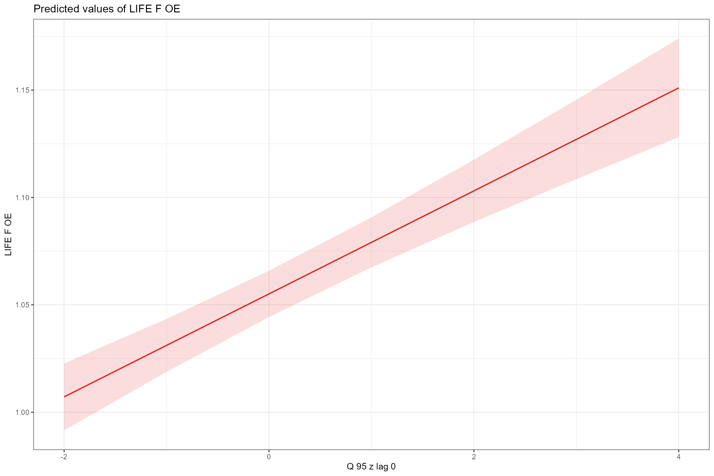
sjPlot::plot_model(model = cs1_mod2,
type = "pred",
pred.type = "fe",
facet.grid = TRUE,
scales = "fixed", terms = "Q95z_lag12")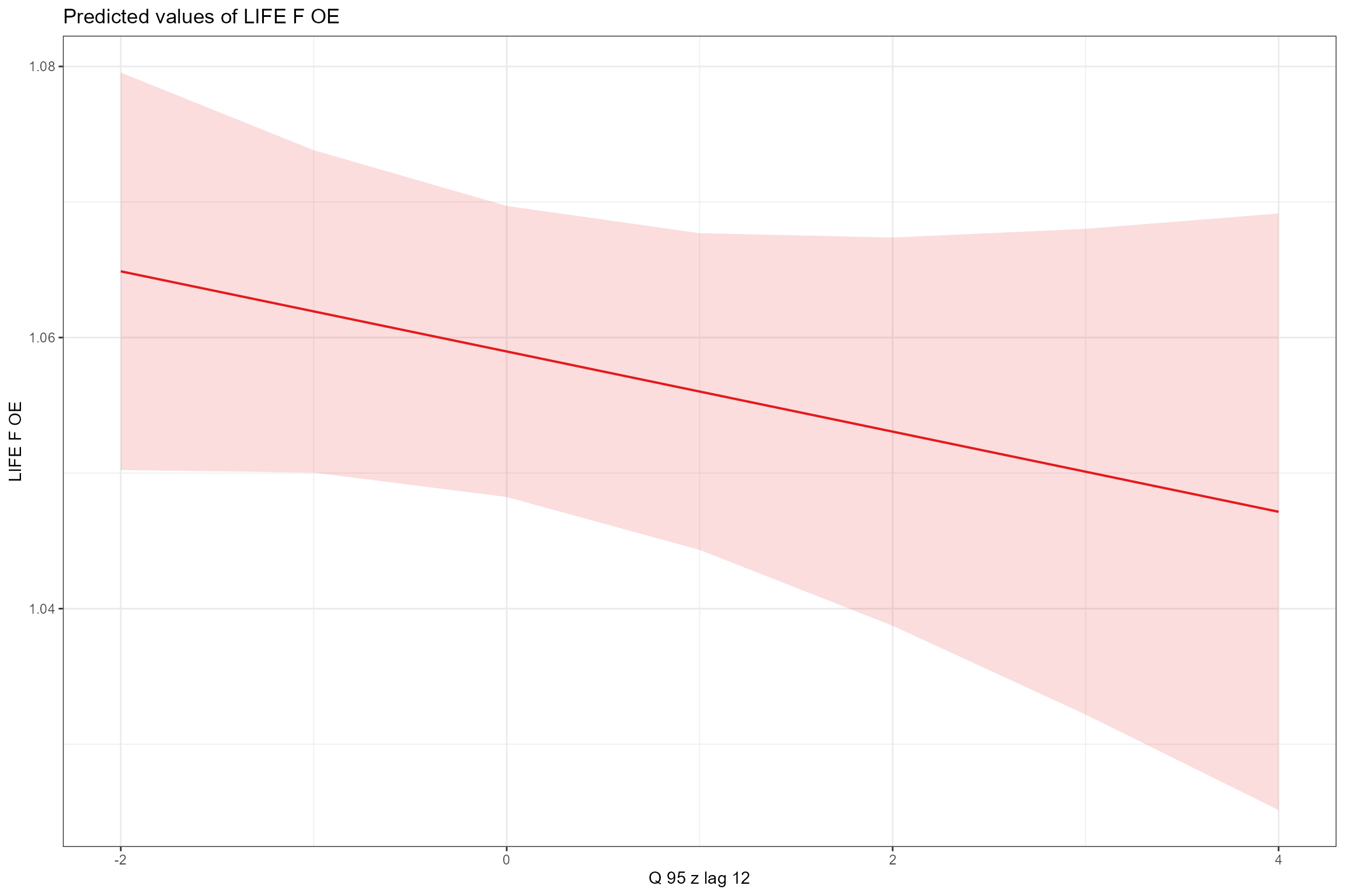
- Interaction plots, for visualising interaction terms. First we examine the interaction between Q95z_lag0 and Season, which shows that LIFE O:E ratios are more sensitive to antecedent Q95 flows in autumn then in spring:
sjPlot::plot_model(model = cs1_mod2,
type = "pred",
terms = c("Q95z_lag0", "Season"))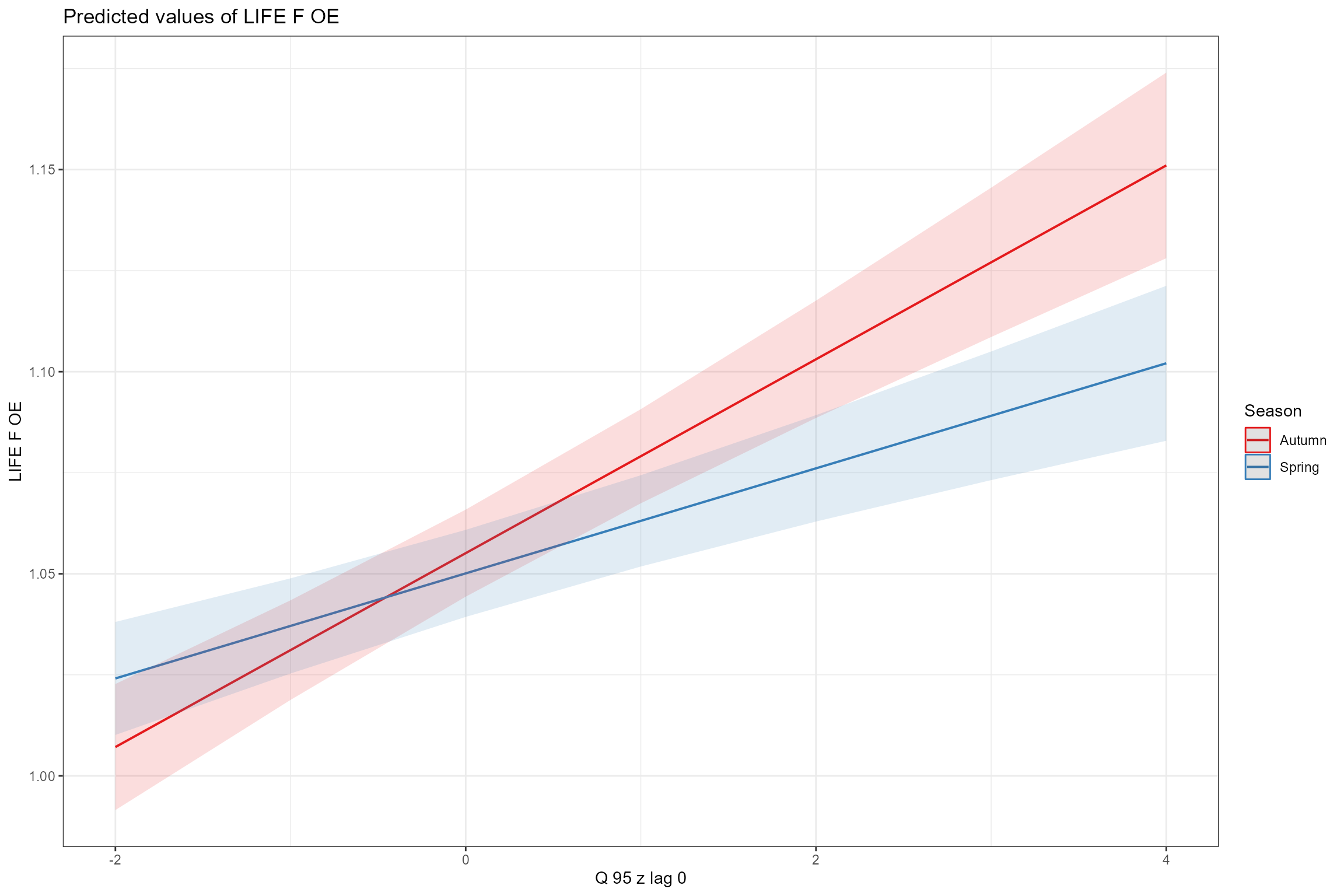
Similarly, the interaction plot for Q95z_lag12 and Season, shows opposing (but very weak) flow effects in the two seasons:
sjPlot::plot_model(model = cs1_mod2,
type = "pred",
terms = c("Q95z_lag12", "Season"))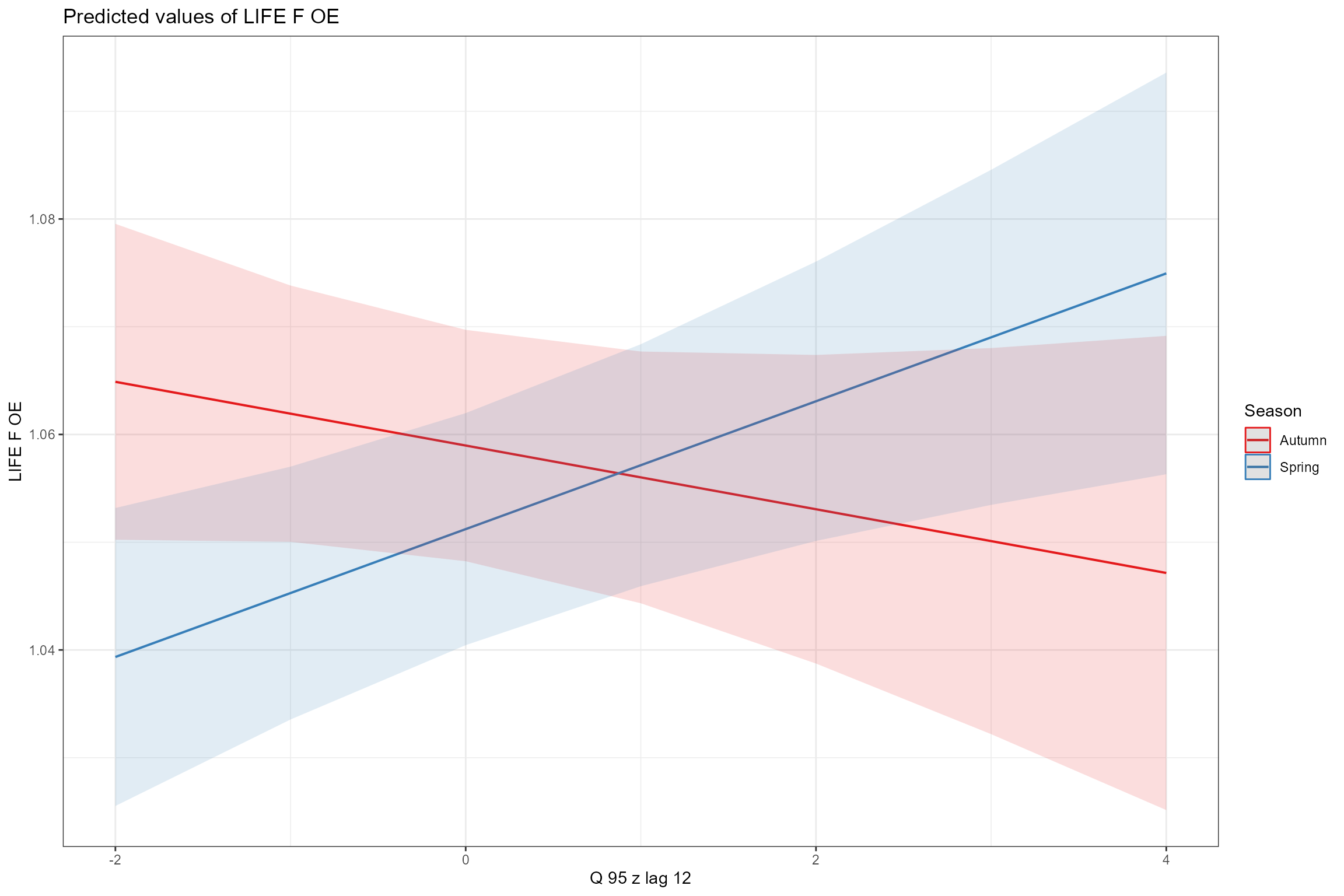
Scenario analysis
Having calibrated a model using the flows experienced historically, we can use the final model to predict the response under alternative flow scenarios. For instance, we can make predictions of LIFE O:E under naturalised flows; the difference between the predictions under historical and naturalised flows then provides a measure of how much abstraction pressure is affecting the macroinvertebrate community.
The final model did not include the flow alteration variable
LTQ95RFR (if it had, this variable could be fixed at 1 to
represent an absence of flow alteration under a naturalised scenario),
but it did include two flow history variables (q95z_lag0
and q95z_lag12). Below we use the
calc_flowstats function to calculate these two Q95 flow
statistics for naturalised flows. The function includes the facility to
standardise the statistics for one flow scenario (specified via
flow_col) using mean and standard deviation flow statistics
from another scenario (specified via ref_col). For example,
if flow_col = naturalised flows and ref_col =
historical flows, then the resulting statistics can be input into a
hydro-ecological model that has previously been calibrated using
standardised historical flow statistics and used to make predictions of
ecological status under naturalised flows.
# Use calc_flowstats() function to calculate Q95z (this may take a few minutes)
cs1_natural_scenario_flowstats <- hetoolkit::calc_flowstats(data = cs1_flowraw_wide,
site_col= "flow_site_id",
date_col= "Date",
flow_col= "Naturalised",
ref_col = "Historical",
imputed_col= NULL,
win_start = "1990-01-01",
win_width = "1 year",
win_step = "1 month",
date_range = NULL)
# Extract data frame of time-varying flow statistics, and select only essential columns
cs1_natural_scenario_flowstats <- cs1_natural_scenario_flowstats[[1]] %>%
dplyr::select("flow_site_id", "win_no", "start_date", "end_date", "Q95z_ref") %>%
dplyr::rename(Q95z = "Q95z_ref")
cs1_historical_scenario_flowstats <- cs1_flowstats[[1]] %>%
dplyr::select("flow_site_id", "win_no", "start_date", "end_date", "Q95z")To generate model predictions for spring (mid-April) and autumn
(mid-October) in every year at every site (not just those that happen to
have a macroinvertebrate sample) we use expand.grid to
create a prediction dataset, and then join it to the naturalised and
historical flow statistics. Note how the prediction datasets contain all
the predictor variables used in the final model.
# Create a prediction data set
cs1_predict_biol_data <- expand.grid(biol_site_id = unique(cs1_biol_all$biol_site_id),
Year = seq(1995,2018), Season = c("Spring", "Autumn"))
cs1_predict_biol_data <- cs1_predict_biol_data %>%
# Center the year to 2005
dplyr::mutate(Year_2005 = Year - 2005) %>%
# Create date column for joining in flow statistics
dplyr::mutate(date = ifelse(cs1_predict_biol_data$Season == "Spring",
paste0(cs1_predict_biol_data$Year, "-04-15"),
paste0(cs1_predict_biol_data$Year, "-10-15"))) %>%
dplyr::mutate(date = lubridate::ymd(date))
# Join flow data
cs1_natural_he <- hetoolkit::join_he(biol_data = cs1_predict_biol_data,
flow_stats = cs1_natural_scenario_flowstats,
mapping = cs1_metadata,
lags = c(0, 12),
method = "A",
join_type = "add_flows")
cs1_historical_he <- hetoolkit::join_he(biol_data = cs1_predict_biol_data,
flow_stats = cs1_historical_scenario_flowstats,
mapping = cs1_metadata,
lags = c(0,12),
method = "A",
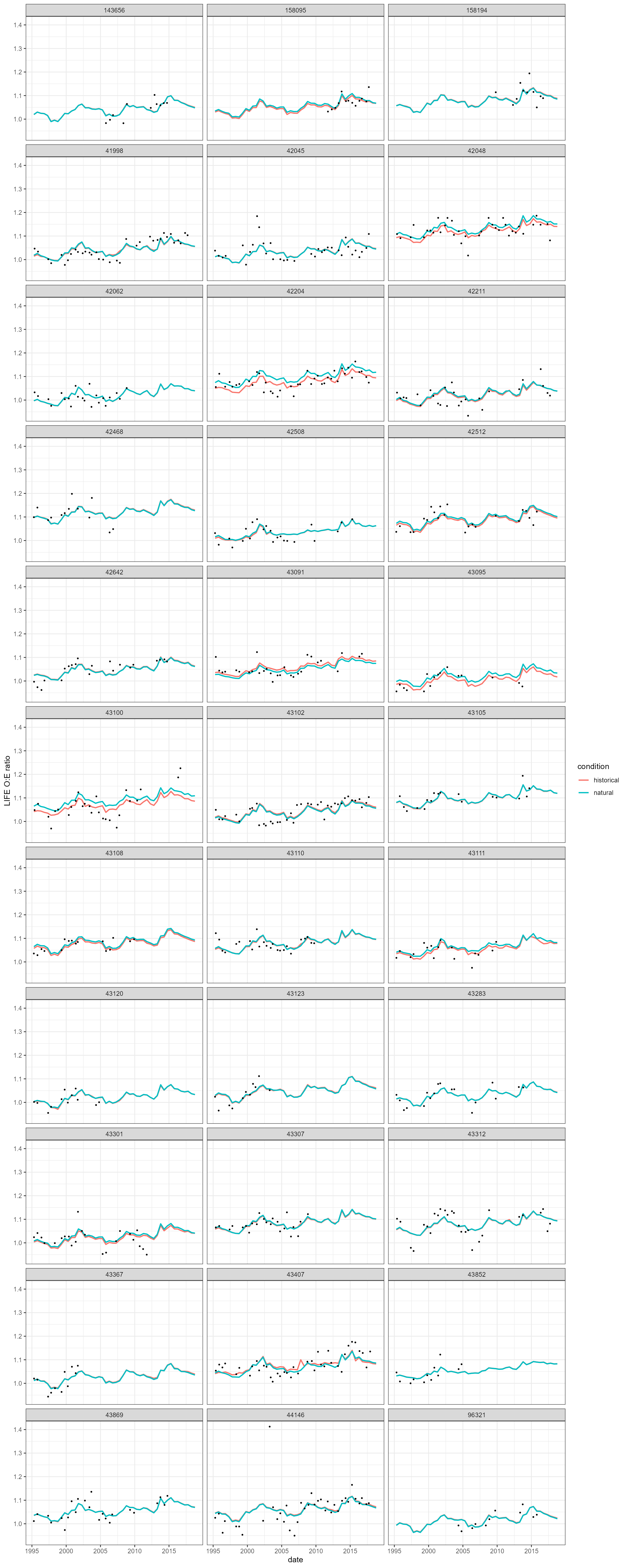
join_type = "add_flows")Now we can use the predict function to predict LIFE O:E
under both the naturalised and historical scenarios, and plot the
results. We can see how the “historical” line describes the patterns in
the historical data (the black points), and interpret the difference
between the historical and naturalised scenarios as the effect of flow
alteration. In this example, the historic and naturalised predictions
are broadly similar, though with some evidence that flow alteration is
suppressing macroinvertebrate LIFE O:E ratios at a handful of sites.
There are also specific cases (e.g. sites 43091 and 43407) where
naturalised predictions of LIFE O:E are lower than historic predictions,
a result of flows being augmented (historic > natural) at these
sites.
# Make predictions
cs1_natural_he$predict <- predict(cs1_mod2, newdata = cs1_natural_he)
cs1_historical_he$predict <- predict(cs1_mod2, newdata = cs1_historical_he)
# Create a data frame with the predicted values, biol_site_id, date and scenario
# (natural or historical), ready for plotting
cs1_predicted_data <- rbind(
data.frame(value = cs1_natural_he$predict, condition = "natural",
biol_site_id = cs1_natural_he$biol_site_id, date = cs1_natural_he$date),
data.frame(value = cs1_historical_he$predict, condition = "historical",
biol_site_id = cs1_historical_he$biol_site_id, date = cs1_historical_he$date)
)
# Plot the predictions, with the true (measured) values as points for reference.
ggplot(cs1_predicted_data, aes(x = date, y = value, color = condition)) +
geom_line(size = 0.8) +
geom_point(data = cs1_biol_all, aes(x = date, y = LIFE_F_OE, color = "measured"),
size = 0.5, colour = "black") +
facet_wrap(~ biol_site_id, ncol = 3) +
labs(y = "LIFE O:E ratio") +
theme_bw()