Macrophytes in chalk streams

Introduction

This case study focuses on a macrophyte dataset of 58 sampling locations on the Test and Itchen (T&I), two groundwater-fed Chalk rivers in Hampshire, England. In particular, it illustrates the use of water quality data and modelled flow data within a hydro-ecological model.

Sites were included in the model calibration dataset if they met all of the following criteria:

At least 3 macrophyte surveys within the time period covered by the flow data.
The site is not on a side channel where flow is controlled by hatches/sluices.
The site is located on a reach with perennial flow (defined as natural Q99 > 0).
The site is not subject to overwhelming artificial physical modifications (e.g. dredged channel, upstream of a weir).
The site has no major water quality issues.
The site is not subject to some other, potentially over-riding, pressure.
The site has no history of major habitat restoration work.

Historical flows at each sampling location were modelled using the EA’s T&I regional groundwater model. Naturalised flows were also modelled by turning off the effect of abstraction and discharges. Using these two flow time series, the case study explores if and how the macrophyte community (as indexed by the RMHI and RMNI metrics) is affected long-term flow alteration, whilst also controlling for natural hydrological variability (flow history) and changes in water quality.

As this case study is intended to illustrate the application of the HE toolkit, rather than be a comprehensive analysis in its own right, some of the analytical steps have been simplified for brevity.

This case study is optimised for viewing in Chrome.

Set-up

Install and load the HE Toolkit:

Install and load the other packages necessary for this case study:

if(!require(pacman)) install.packages("pacman")
pacman::p_load(knitr, DT, GGally, sf, ggfortify, plyr, lmerTest)

## Set ggplot theme
theme_set(theme_bw())

Metadata file

We start by importing a “metadata” file with the following columns: * biol_site_id = Macrophyte sampling site ID * flow_site_id = ID’s for paired sites with modelled flow data available * wq_site_id = Water quality site ID

These id’s are subsequently used to download data from the Environment Agency’s (EA) Ecology and Fish Data Explorer (EDE) and Water Quality Archive, and to join disparate datasets together.

# Load in the metadata file 
cs3_metadata <- readxl::read_excel("Data/CaseStudy3/cs3_metadata.xlsx")

# make all columns character vectors 
cs3_metadata$biol_site_id <- as.character(cs3_metadata$biol_site_id)
cs3_metadata$flow_site_id <- as.character(cs3_metadata$flow_site_id)
cs3_metadata$wq_site_id <- as.character(cs3_metadata$wq_site_id)

# Get site lists for later use in functions: 
cs3_biolsites <- cs3_metadata$biol_site_id
cs3_flowsites <- cs3_metadata$flow_site_id
cs3_wq_site_id <- cs3_metadata$wq_site_id

Macrophyte data

Import macrophyte data

Macrophyte data has to be manually downloaded from the Environment Agency’s Ecology Data Explorer website as the HE Toolkit does not currently include a fucntion of importing macrophyte survey data. The data is then manually imported and filtered down to the sites listed in the metadata table.

The data includes two macrophyte metrics that are candidate response variables:

River Macrophyte Hydraulic Index (RMHI) This is a measure of which plants grow in the river and their association with flow. It is measured on a scale from 1-10, where high scores are associated with species that grow in low flow energies.

River Macrophyte Nutrient Index (RMNI) This is a measure of which plants grow in the river and their association with high nutrients. It is measured on a scale from 1-10, where high scores are associated with species that dominate under nutrient enriched conditions.

# read in macrophyte data
cs3_biol_data <- read.csv("Data/CaseStudy3/EA_download/macp_data_metrics.csv")

cs3_biol_data <- cs3_biol_data %>%
  dplyr::select(SITE_ID, NGR_10_FIG, SAMPLE_DATE, SAMPLE_DATE_YEAR, RMHI, RMNI) %>%
  dplyr::rename(biol_site_id = SITE_ID,
                 date = SAMPLE_DATE, 
                 year = SAMPLE_DATE_YEAR) %>%
  dplyr::mutate(date = as.Date(date, format = "%Y-%m-%d"))%>%
  dplyr::mutate(biol_site_id = as.character(biol_site_id))

# Remove sites in biol_data that are not in the metadata
cs3_biol_data <- subset(cs3_biol_data, biol_site_id %in% cs3_metadata$biol_site_id) 

#Remove sites where there are less that 3 macrophyte samples
cs3_biol_all <- cs3_biol_data %>%
  dplyr::group_by(biol_site_id) %>%
  dplyr::filter(n() >= 3) %>%
  dplyr::ungroup()

# Remove sites where the RMNI and RMHI are NA
cs3_biol_all <- cs3_biol_all[complete.cases(cs3_biol_all$RMNI,
cs3_biol_all$RMHI), ]

View the filtered macrophyte data:

Visualise macrophyte data

The following exploratory plots show:

A Histogram of RMHI and RMNI scores
The total number of surveys per year

ggplot(data = cs3_biol_all, aes(x = RMNI)) +
  geom_histogram() +
  xlab("River Macrophyte Hydrualic Index (RMHI)") +
  ylab("Count") +
  ggtitle("Histogram of RMHI scores")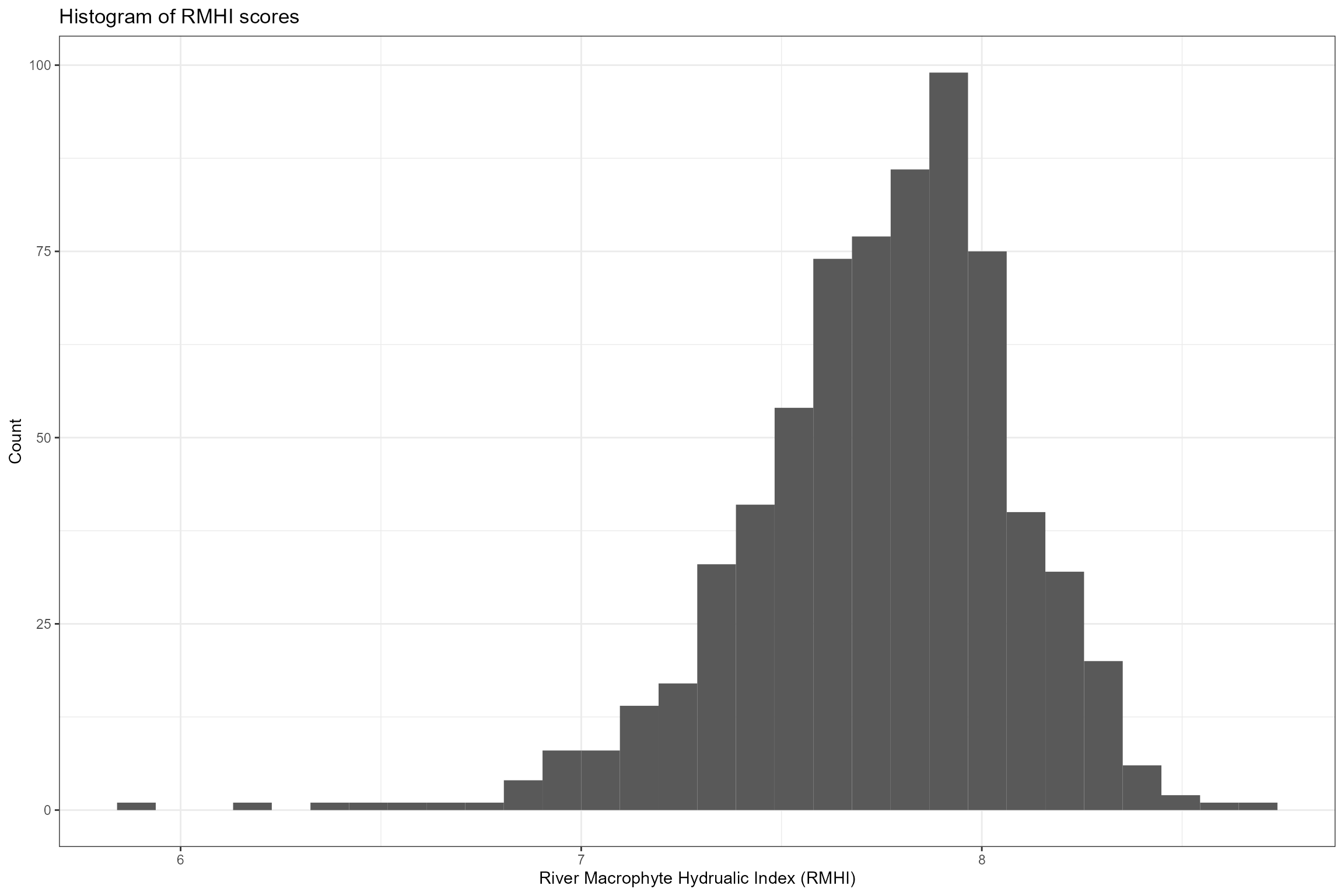

ggplot(data = cs3_biol_all, aes(x = RMHI)) +
  geom_histogram() +
  xlab("River Macrophyte Nutrient Index (RMNI)") +
  ylab("Count") +
  ggtitle("Histogram of RMNI scores")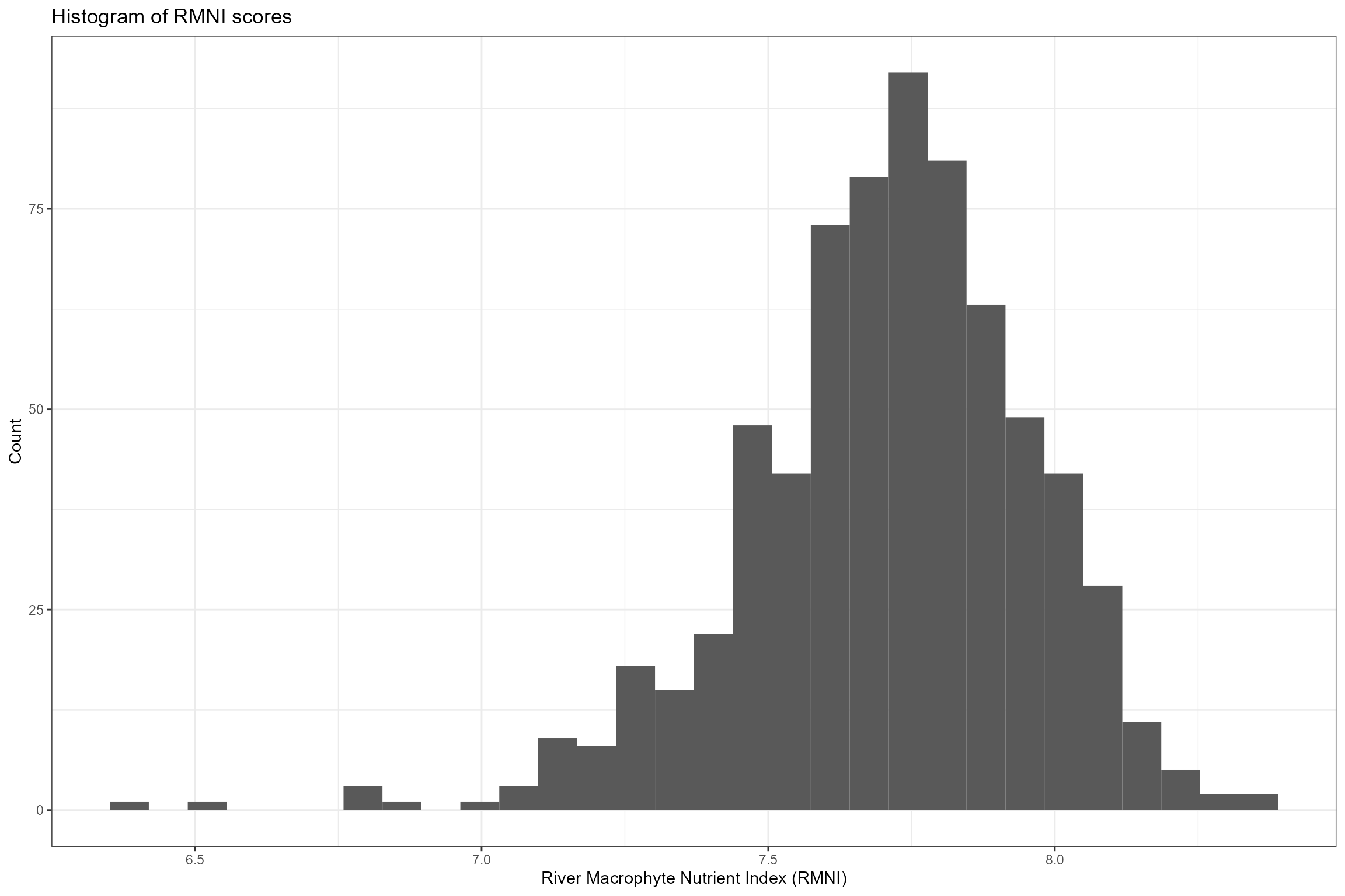

# Convert date variable to year
cs3_biol_all$year <- lubridate::year(cs3_biol_all$date)

# Count the number of samples per year
samples_per_year <- cs3_biol_all %>% 
  dplyr::group_by(year) %>% 
  dplyr::summarise(num_samples = n())

# Create bar chart of number of macrophyte surveys per year
ggplot(data = samples_per_year, aes(x = year, y = num_samples)) +
  geom_bar(stat = "identity") +
  xlab("Year") +
  ylab("Number of surveys") +
  ggtitle("Total mumber of surveys per year")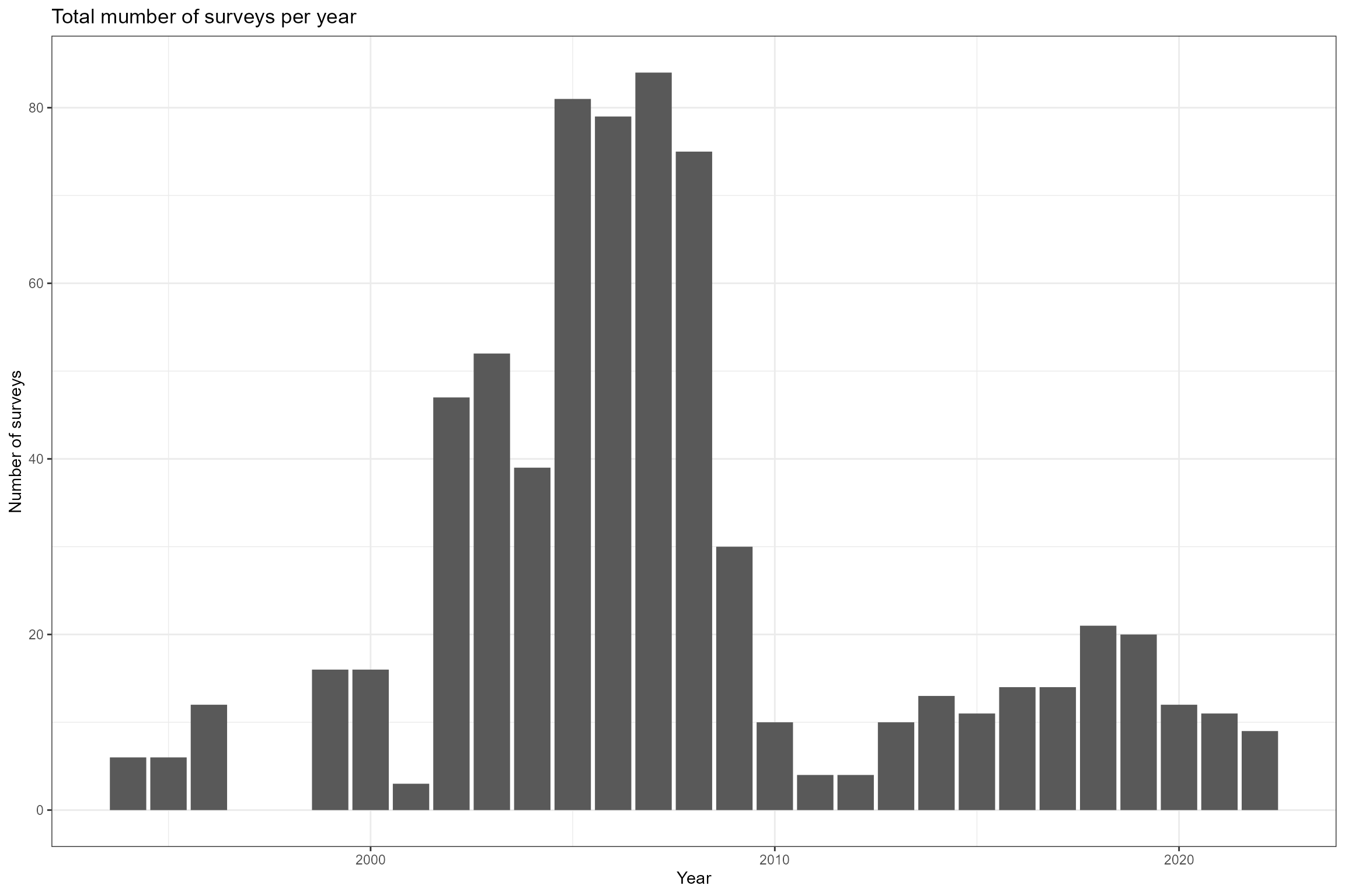

Water quality data

Import data

Below, we use the import_wq function and our list of wq_site_ids to import water quality sample data from the Environment Agency’s Water Quality Archive database. The Water Quality Data Archive only holds data since 2000, so we also manually import additional water quality data from 1993-1999, and then join the two datasets together. Macrophytes are sensitive to the degree of nutrient enrichment, so we choose to focus on orthophosphate (EA det code 180) as measure the amount of biologically available phosphorus in the water column.

# Import water quality data from 2000 onwards
cs3_wq <- hetoolkit::import_wq(sites = cs3_wq_site_id, start_date = "1993-01-01", end_date = "2022-12-31", dets = 180)

# Import additional water quality data pre-2000
cs3_additional_wq <- readRDS("Data/CaseStudy3/cs3_additional_wq.rds")

# Join the two datasets 
cs3_wq <- rbind(cs3_wq, cs3_additional_wq)

# Create a year variable: 
cs3_wq <- cs3_wq %>%
  dplyr::mutate(year = lubridate::year(date))

View the imported water quality data:

Explore data

We plot the sample data as a time series for each site to check for significant step changes or trends. Note that there are just 26 unique water quality sites linked to the 58 macrophyte sites. Some sites show strong declining trends in orthophosphate concentration, so time-varying statistics are likely to be more useful than long-term statistics.

cs3_wq %>%
  dplyr::filter(det_label == "Orthophospht") %>%
  ggplot(aes(x = date, y = result)) + 
    geom_point(size=0.1) +
    ylab("Orthophospht concentration (mg/l)") +
    xlab("") +
    facet_wrap(~ wq_site_id, scales = "free_y", ncol = 5)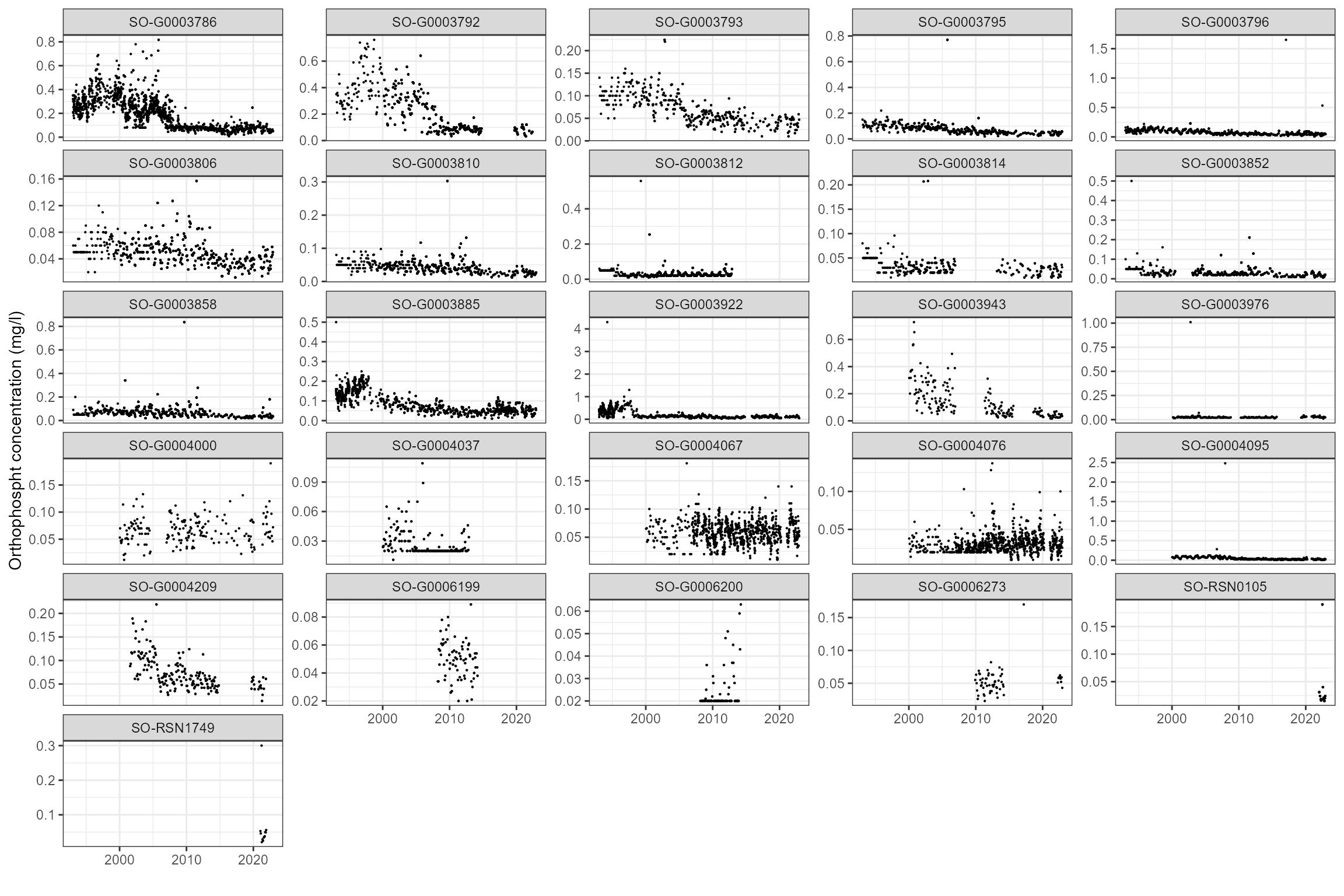

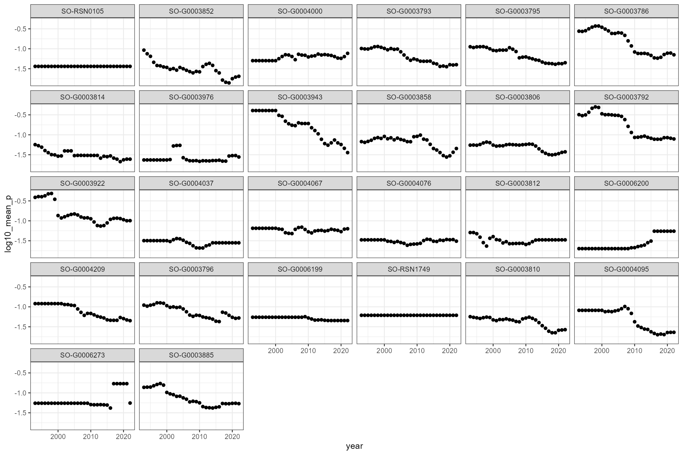
Summarise data

Following the Water Framework Directive (WFD) approach to classification, we choose to calculate the mean orthophosphate concentration for a rolling three year period at each site.

# Calculate rolling 3-year summary statistics, by site and id. 
cs3_wq_summary <- expand.grid(year = seq(from = 1993, to = 2022), wq_site_id = unique(cs3_metadata$wq_site_id))

for(i in 1:dim(cs3_wq_summary)[1]){

  # Filter down to rolling three year window
  temp <- cs3_wq %>%
    dplyr::filter(year <= cs3_wq_summary$year[i] & year >= cs3_wq_summary$year[i]-2)
  
  # Calculate mean orthophsophate
  cs3_wq_summary$mean_p[i] <- mean(temp$result[temp$det_label == "Orthophospht" & temp$wq_site_id == cs3_wq_summary$wq_site_id[i]], na.rm = TRUE)

  rm(temp)
  
}

# Infill NAs using values for neighbouring years
cs3_wq_summary <- cs3_wq_summary %>%
  dplyr::group_by(wq_site_id) %>%
  tidyr::fill(mean_p, .direction = "downup") %>%
  dplyr::ungroup()

# Finally, the rolling average orthophosphate data are skewed so we apply a log-10 transformation 
cs3_wq_summary <- cs3_wq_summary %>%
 dplyr::mutate(log10_mean_p = log10(mean_p))

These are the resulting rolling three-year summary statistics for each water quality site:

Flow data

Modelled time series of historical and naturalised flows on a 7-daily time step were exported from the Test and Itchen (T&I) groundwater model for the period 1965-2017. (Estimated flows under Recent Actual and Fully Licensed conditions were also available but not used). Note that there are 55 unique flow sites (stream cells) linked to the 58 macrophyte sites.

The data, stored as an RDS file, were then manually imported into R:

Import data

cs3_flowraw_long <- readRDS("Data/CaseStudy3/cs3_flows.rds")

# Convert to wide format (one column for each flow scenario)
cs3_flowraw_wide <- cs3_flowraw_long %>% 
  tidyr::pivot_wider(names_from = Scenario, values_from = flow)

Look at the long and wide format of the flow data:

## # A tibble: 6 × 6
##   flow_site_id Date         flow Scenario   `__index_level_0__` model
##   <chr>        <date>      <dbl> <chr>                    <int> <chr>
## 1 TI7501       1985-01-02  2710. Historical             4333783 TI   
## 2 TI7607       1985-01-02  2780. Historical             4333794 TI   
## 3 TI9898       1985-01-02  9292. Historical             4333950 TI   
## 4 TI10670      1985-01-02  3411. Historical             4334097 TI   
## 5 TI12205      1985-01-02 42321. Historical             4334618 TI   
## 6 TI13070      1985-01-02 71316. Historical             4335067 TI

## # A tibble: 6 × 8
##   flow_site_id Date       `__index_level_0__` model Historical Naturalised
##   <chr>        <date>                   <int> <chr>      <dbl>       <dbl>
## 1 TI7501       1985-01-02             4333783 TI         2710.       3685.
## 2 TI7607       1985-01-02             4333794 TI         2780.       3985.
## 3 TI9898       1985-01-02             4333950 TI         9292.       9323.
## 4 TI10670      1985-01-02             4334097 TI         3411.       4271.
## 5 TI12205      1985-01-02             4334618 TI        42321.      42428.
## 6 TI13070      1985-01-02             4335067 TI        71316.      71190.
## # ℹ 2 more variables: RecentActual <dbl>, FullyLicensed <dbl>

Visualise data

The following plots show the modelled historical and naturalized flows at each monitoring location.

cs3_ti_data <- cs3_flowraw_long %>%
  dplyr::filter(Scenario %in% c("Historical", "Naturalised")) %>%
  split(.$Scenario)

plot_list <- lapply(cs3_ti_data, function(data) {
  ggplot(data, aes(x = Date, y = flow))+
    geom_line(aes(colour = Scenario), size = 1)+
    ggthemes::scale_colour_colorblind()+
    facet_wrap(~ flow_site_id)+
    xlab("Year") +
    ylab("Flow Ml/d")
})

# Combine plots into one grid
gridExtra::grid.arrange(grobs = plot_list, ncol = 2)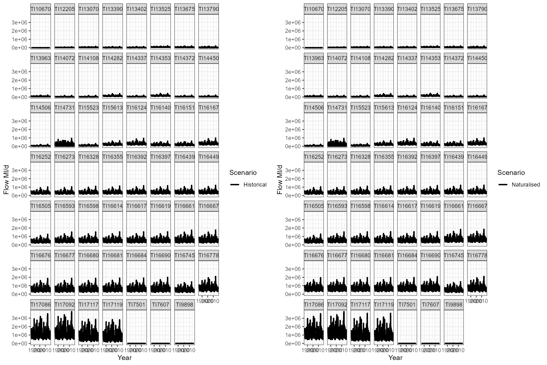

Calculate flow statistics

The flow data were processed to calculate, for each site, (i) the degree of long-term flow alteration, and (ii) a time-varying metric of flow history, designed to capture the effect of inter-annual variation in flow.

Flow alteration metric

To quantify the degree of abstraction pressure at each site, the long-term historical Q95 was calculated and expressed as a ratio of the long-term naturalised Q95 to yield a long-term Q95 Residual Flow Ratio (RFR) variable. A ratio of 1 indicates that were flows are not influenced (i.e. at natural); ratios <1 indicate a progressively greater degree of abstraction pressure (i.e. flow reduction), and a ratios >1 indicates that flows are higher than natural (i.e. the watercourse is discharge-rich).

We first calculate a time series of annual RFRs for each site, to check whether the degree of flow alteration has changed over time:

# Calculate and plot annual flow alteration statistics for each site

cs3_flowraw_wide$Year <- year(cs3_flowraw_wide$Date)

cs3_flowraw_wide %>%
  group_by(flow_site_id, Year) %>% 
  dplyr::summarise(LTQ95hist = quantile(Historical, 0.05, na.rm=TRUE),
                   LTQ95nat = quantile(Naturalised, 0.05, na.rm=TRUE)) %>%
  dplyr::mutate(LTQ95RFR = LTQ95hist / LTQ95nat) %>%
  ggplot(aes(x = Year, y = LTQ95RFR)) +
    geom_line() +
    facet_wrap(~flow_site_id, nrow = 8) +
    labs(x = "Year", y = "Residual Flow Ratio at Q95") +
    theme_bw()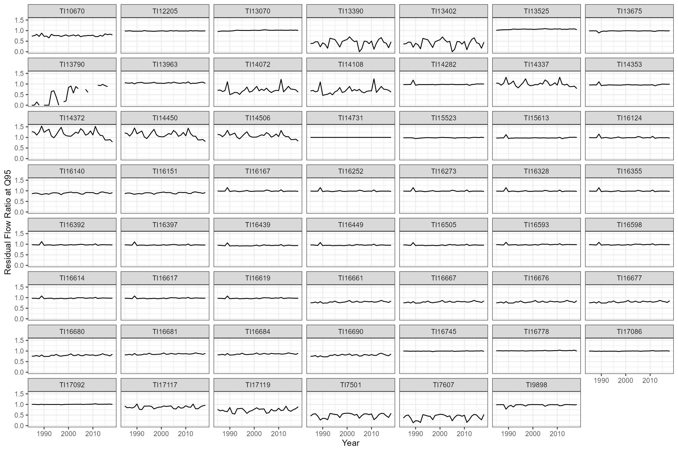

There is inter-annual variability in the degree of flow alteration at some sites, but no evidence of long-term trends that might indicate systematic changes in abstraction pressure. We therefore choose to calculate a long-term RFR for each site (termed LTQ95RFR) and use this in our model as a measure of flow alteration.

# Calculate long-term flow alteration statistics for each site
cs3_rfr <- cs3_flowraw_wide %>%
  dplyr::group_by(flow_site_id) %>% 
  dplyr::summarise(LTQ95hist = quantile(Historical, 0.05, na.rm=TRUE),
                   LTQ95nat = quantile(Naturalised, 0.05, na.rm=TRUE)) %>%
  dplyr::mutate(LTQ95RFR = LTQ95hist / LTQ95nat)

cs3_rfr$LTQ95RFR[is.nan(cs3_rfr$LTQ95RFR)] <- 0

Flow history metric

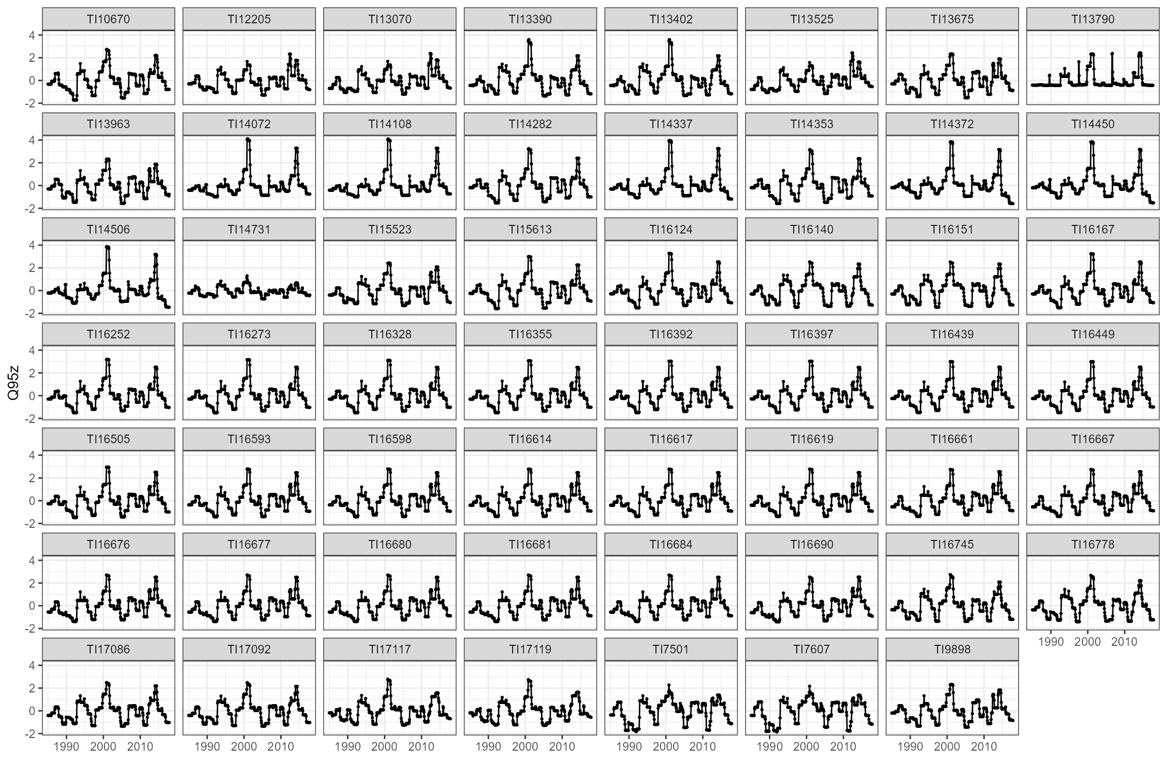
The calc_flowstats function takes a time series of a measured or modelled flows and uses a user-defined moving window to calculate a suite of time-varying flow statistics for one or more sites. Below, calc_flowstats is used to calculate the Q95 for a moving 12 month window at a one month time step. The Q95 values are then standardised to make them dimensionless and comparable among sites.

# Set any negative flow values to NA's 
cs3_flowraw_wide$Historical[cs3_flowraw_wide$Historical <= 0] <- NA

# Use calc_flowstats() function to calculate Q95z (this may take a few minutes)
cs3_flowstats <- hetoolkit::calc_flowstats(data = cs3_flowraw_wide,
                                           site_col= "flow_site_id",
                                           date_col= "Date",
                                           flow_col= "Historical",
                                           imputed_col= NULL,
                                           win_start = "1985-01-01",
                                           win_width = "1 year",
                                           win_step = "1 month",
                                           date_range = NULL)

# Extract data frame of time-varying flow statistics, and select only essential columns
cs3_flowstats1 <- cs3_flowstats[[1]] %>%
  dplyr::select("flow_site_id", "win_no", "start_date", "end_date", "Q95z")

# Remove rows where Q95z is NA
cs3_flowstats1 <- cs3_flowstats1[complete.cases(cs3_flowstats1$Q95z), ]

cs3_flowstats1$flow_site_id <- as.factor(cs3_flowstats1$flow_site_id)

cs3_flowstats2 <- cs3_flowstats[[2]]

Visualise the standardised time-varying Q95 statistics:

Join hydrological and ecological data

The join_he function links biology (in this case macrophyte) data with time-varying flow statistics for one or more antecedent (lagged) time periods (as calculated by the calc_flowstats function above) to create a combined dataset for hydro-ecology modelling. Here we use method = "A" and lags = c(0, 12, 24) to get the annual flow statistics for three years priors to each macrophyte survey. For example, a macrophyte sample collected in April 2015 will be joined with flow statistics for the periods April 2014-March 2015 (lag 0) and April 2013-March 2014 (lag 12) and April 2012-March 2013 (lag 24).

cs3_he1 <- hetoolkit::join_he(biol_data = cs3_biol_all,
                              flow_stats = cs3_flowstats1,
                              mapping = cs3_metadata,
                              lags = c(0,12,24),
                              method = "A", 
                              join_type = "add_flows") %>%

# Manually join the long-term flow alteration statistics and water quality statistics for each site
  dplyr::left_join(cs3_rfr, by = "flow_site_id") %>%
  dplyr::left_join(cs3_wq_summary, by = c("wq_site_id","year")) 

# Separately, join the macrophyte data to the time-varying flow statistics to create a dataset for data visualisation (this feeds into the plot_rngflows function below)
cs3_he2 <- hetoolkit::join_he(biol_data = cs3_biol_all,
                              flow_stats = cs3_flowstats1,
                              mapping = cs3_metadata,
                              lags = c(0,12,24),
                              method = "A", 
                              join_type = "add_biol")

View the first dataset created using join_type = "add_flows":

And now the second dataset created using join_type = "add_biol":

Modelling

Assess coverage of historical flow conditions

The plot_rngflows function generates a scatterplot for two flow variables and overlays two convex hulls: one showing the full range of flow conditions experienced historically, and a second convex hull showing the range of flow conditions with associated biology samples. This visualization helps identify to what extent the available biology data span the full range of flow conditions experienced historically.

In the following example, we plot the Q95z flow statistics in each of the previous two years, for all sites combined. In this example, the orange polygon almost completely fills the grey polygon, indicating that the biology samples provide excellent coverage of historical flow conditions.

hetoolkit::plot_rngflows(data = cs3_he2, 
                         flow_stats = c("Q95z_lag0","Q95z_lag12"), 
                         biol_metric = "RMHI")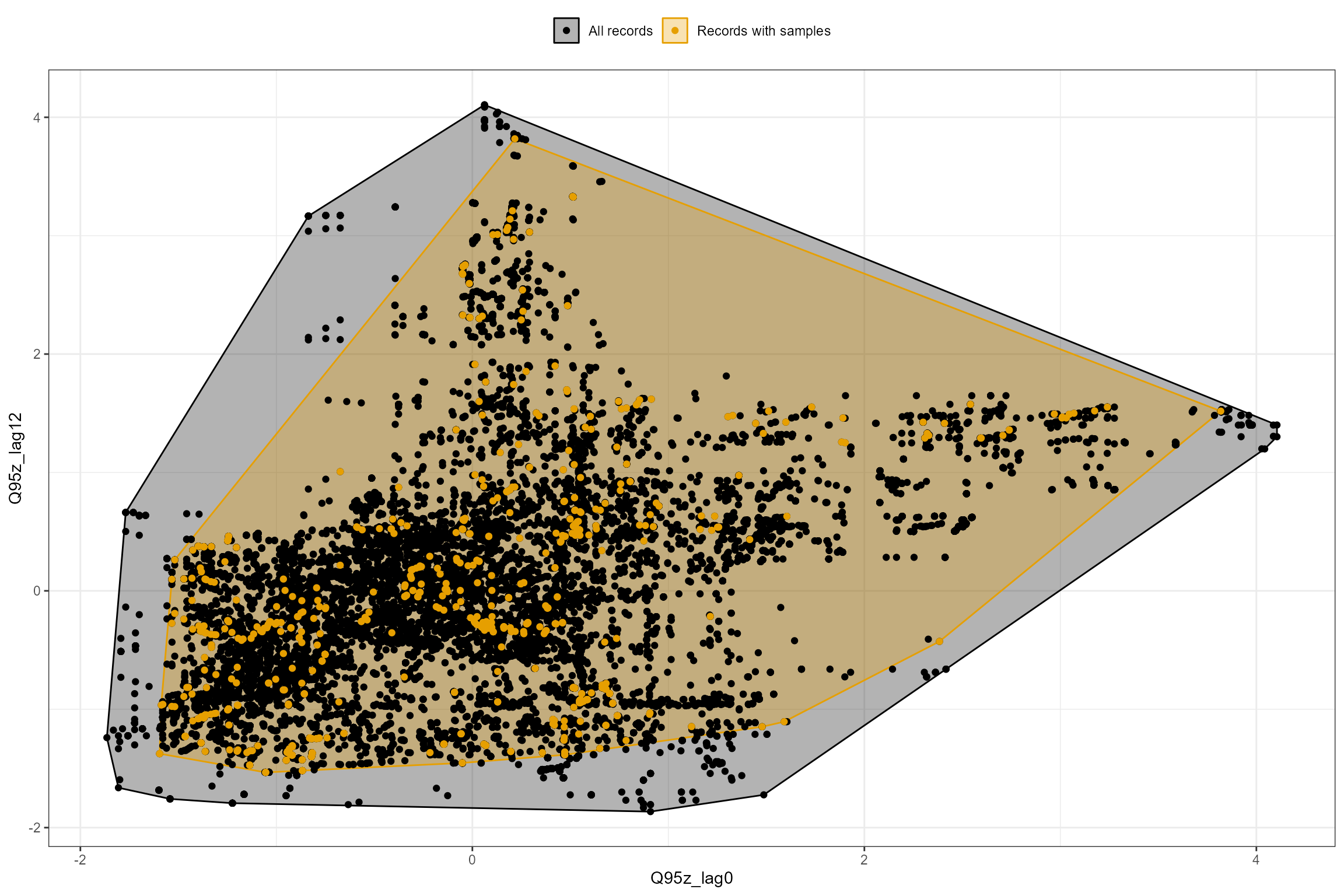

Data preparation

We use pairwise plots to identify highly correlated variables (that might need to be excluded as candidate predictor variables), skewed variables (that might benefit from transformation), and gross outliers (none found).

# produce pairs plot
cs3_he1 %>%
  dplyr::select(year, LTQ95RFR, log10_mean_p, Q95z_lag0, Q95z_lag12, Q95z_lag24, RMHI, RMNI) %>%
  GGally::ggpairs(lower = list(continuous = "smooth_loess"))

To aid model convergence, we also center the year variable to the approximate mid-point of the dataset:

cs3_he1 <- cs3_he1 %>%
  dplyr::mutate(Year_2005 = year - 2005)

Model calibration

Using a linear mixed-effects model fitted via the lme4::lmer() function, we model the spatial variation in the RMHI and RMNI metrics as a function of the long term flow alteration (LTQ95RFR), and temporal variation in RMHI and RMNI as a function of flow history over the preceding 1-12 months (Q95z_lag0), 13-24 months (Q95z_lag12) and 25-36 months (Q95z_lag24).

In addition, log10_mean_p was included as a main effect to represent general water quality over the previous three years. (We used a 3 year moving window to mirror the WFD rolling classification process, however further analysis could be undertaken to compare how sensitive results are to differing window widths.). Year_2005 (year, centered so that 2005 = 0) was also included to account for long-term trends unrelated to general water quality, (insofar as these are represented by the log10_mean_p variable).

Site (biol_site_id) was included as a random intercept to measure spatial variation in RMHI and RMNI that cannot be explained by patterns in flow alteration and water quality. It was not possible to fit any random slopes because there were too few macrophyte surveys per site (an average of 12 per site).

The RMHI and RMNI metrics are very strongly correlated (r = 0.82, as shown in the pairs plot above) and so, not surprisingly, the RMHI and RMNI models produced very similar results. For brevity we show only the RMHI model here.

First we fit a full model containing all of these terms. Note the use of the lmerTest package, which provides approximate p-values for fixed effects in summary():

# fit full model using the lmerTest package
cs3_mod1 <- lmerTest::lmer(RMHI ~ 
                     Year_2005 +
                     LTQ95RFR +
                     Q95z_lag0 +
                     Q95z_lag12 +
                     Q95z_lag24 +
                     log10_mean_p +
                     (1 | biol_site_id),
                    data = cs3_he1,
                    REML = FALSE, 
                   control = lmerControl(optimizer="bobyqa", optCtrl = list(maxfun = 10000)))

summary(cs3_mod1)

## Linear mixed model fit by maximum likelihood . t-tests use Satterthwaite's
##   method [lmerModLmerTest]
## Formula: RMHI ~ Year_2005 + LTQ95RFR + Q95z_lag0 + Q95z_lag12 + Q95z_lag24 +  
##     log10_mean_p + (1 | biol_site_id)
##    Data: cs3_he1
## Control: lmerControl(optimizer = "bobyqa", optCtrl = list(maxfun = 10000))
## 
##      AIC      BIC   logLik deviance df.resid 
##   -299.5   -258.4    158.8   -317.5      700 
## 
## Scaled residuals: 
##     Min      1Q  Median      3Q     Max 
## -4.0892 -0.4757  0.0742  0.6116  3.8604 
## 
## Random effects:
##  Groups       Name        Variance Std.Dev.
##  biol_site_id (Intercept) 0.03688  0.1920  
##  Residual                 0.03020  0.1738  
## Number of obs: 709, groups:  biol_site_id, 58
## 
## Fixed effects:
##                Estimate Std. Error         df t value Pr(>|t|)    
## (Intercept)    7.754259   0.123110  81.335198  62.987   <2e-16 ***
## Year_2005     -0.004427   0.002263 581.652195  -1.956   0.0509 .  
## LTQ95RFR       0.037779   0.122151  64.464644   0.309   0.7581    
## Q95z_lag0      0.008437   0.008752 654.870645   0.964   0.3354    
## Q95z_lag12     0.016750   0.009045 654.236702   1.852   0.0645 .  
## Q95z_lag24     0.038882   0.009628 675.554809   4.038    6e-05 ***
## log10_mean_p   0.038689   0.058310 330.219089   0.664   0.5075    
## ---
## Signif. codes:  0 '***' 0.001 '**' 0.01 '*' 0.05 '.' 0.1 ' ' 1
## 
## Correlation of Fixed Effects:
##             (Intr) Y_2005 LTQ95R Q95z_0 Q95_12 Q95_24
## Year_2005    0.098                                   
## LTQ95RFR    -0.798  0.091                            
## Q95z_lag0   -0.030  0.184  0.052                     
## Q95z_lag12  -0.005  0.076  0.001 -0.469              
## Q95z_lag24  -0.057  0.140  0.029  0.295 -0.549       
## log10_men_p  0.443  0.405  0.140  0.035 -0.003 -0.037

The p-values from summary() are only approximate and cannot be relied upon to guide model selection. Nonetheless, some of the terms appear to be non-significant, suggesting that some model simplification may be beneficial.

Next we use the HE Toolkit’s model_logocv function to perform cross validation and guide a backwards elimination process with the goal of identifying a more parsimonious model. Cross validation - testing how well the model is able to predict RMHI at each site in turn when that site is dropped from the calibration dataset - provides a robust measure of the model’s predictive performance (quantified as the Root Mean Square Error, or RMSE), and can be used to identify and eliminate unimportant variables. In this case study, the primary focus is on assessing the influence of flow alteration on spatial patterns in RMHI and so we choose to use the model_logocv function, which puts more emphasis on the model’s ability to explain spatial variation, over the model_cv function, which puts more emphasis on temporal variation.

Note that to use the model_logocv function, models need to be fitted using the lme4 (not lmerTest) package.

Model simplification is conducted in a stepwise manner, with one term being eliminated at a time, until no further improvement in the RMSE can be achieved. Following this process (not shown for brevity), the final model is:

#fit final model
cs3_mod_final <- lme4::lmer(RMHI ~ 
                    Year_2005 +
                   # LTQ95RFR +
                   Q95z_lag0 +
                   Q95z_lag12 +
                   Q95z_lag24 +
                  #  log10_mean_p +
                    (1|biol_site_id),
                    data = cs3_he1,
                    REML = FALSE, 
                   control = lmerControl(optimizer="bobyqa", optCtrl = list(maxfun = 10000)))

# calculate RMSE for the final model
cs3_mod_final_logocv <- hetoolkit::model_logocv(model = cs3_mod_final, 
                                           data = cs3_he1, 
                                           group = "biol_site_id",
                                           control = lmerControl(optimizer="bobyqa", optCtrl = list(maxfun = 10000)))

Comparing the RMSE values for the full and final models:

# full model
cs3_mod1_logocv[[1]]

## [1] 0.2538039

# final model (slightly lower RMSE, so is the preferred model)
cs3_mod_final_logocv[[1]]

## [1] 0.2522514

Model interpretation

## Linear mixed model fit by maximum likelihood . t-tests use Satterthwaite's
##   method [lmerModLmerTest]
## Formula: RMHI ~ Year_2005 + Q95z_lag0 + Q95z_lag12 + Q95z_lag24 + (1 |  
##     biol_site_id)
##    Data: cs3_he1
## Control: lmerControl(optimizer = "bobyqa", optCtrl = list(maxfun = 10000))
## 
##      AIC      BIC   logLik deviance df.resid 
##   -303.0   -271.1    158.5   -317.0      702 
## 
## Scaled residuals: 
##     Min      1Q  Median      3Q     Max 
## -4.0864 -0.4838  0.0754  0.6072  3.8689 
## 
## Random effects:
##  Groups       Name        Variance Std.Dev.
##  biol_site_id (Intercept) 0.03740  0.1934  
##  Residual                 0.03019  0.1738  
## Number of obs: 709, groups:  biol_site_id, 58
## 
## Fixed effects:
##               Estimate Std. Error         df t value Pr(>|t|)    
## (Intercept)   7.741475   0.027475  60.497857 281.764  < 2e-16 ***
## Year_2005    -0.005056   0.002070 557.319468  -2.443   0.0149 *  
## Q95z_lag0     0.008141   0.008735 657.865467   0.932   0.3517    
## Q95z_lag12    0.016763   0.009043 654.564484   1.854   0.0642 .  
## Q95z_lag24    0.039056   0.009615 674.932265   4.062 5.44e-05 ***
## ---
## Signif. codes:  0 '***' 0.001 '**' 0.01 '*' 0.05 '.' 0.1 ' ' 1
## 
## Correlation of Fixed Effects:
##            (Intr) Y_2005 Q95z_0 Q95_12
## Year_2005  -0.253                     
## Q95z_lag0  -0.021  0.184              
## Q95z_lag12 -0.010  0.085 -0.469       
## Q95z_lag24 -0.050  0.170  0.296 -0.549

The preferred model with the lowest RMSE score (cs3_mod_final) included the fixed predictors Year_2005, Q95z_lag0, Q95z_lag12 and Q95z_lag24, while the random effects included an intercept varying by site.

There was no evidence that RMHI was influenced by water quality (log10_mean_p) or long-term flow alteration (LTQ95RFR). This may be because because the 58 sites spanned only a narrow pressure gradient; sites with major water quality issues were screened out of the calibration dataset, and at only a handful of sites was the long-term Q95 reduced by more than 50%.

On average, across all sites, there was a weak decreasing (improving) trend in RMHI of ca. -0.005 per year. After accounting for this underlying trend, RMHI was positively associated with all three Q95z flow statistics; the associations were weak, but became stronger and more significant with increasing time lag (i.e. RMHI was associated more strongly with Q95 flows 25-36 months ago than with flows in the immediately preceding 12 months). The finding of a positive relationship is counter-intuitive as higher RMHI scores are associated with species that grow in habitats with lower flow velocities. The inclusion of additional, longer time lags might be warranted to explore whether this is a genuine result or an artefact of the flow statistics used in the model. If we consider it to be genuine we should attempt further interpretation with reference to the morphology of the sites in the model and the identity of the dominant macrophyte species driving the RMHI response.

Model diagnostics

The diag_lmer function produces a variety of diagnostic plots for a mixed-effects regression (lmer) model. Below we create model diagnostic plots for the final model (cs3_mod_final).

# generate diagnostic plots 
cs3_diag_plots <- hetoolkit::diag_lmer(
 model = cs3_mod_final, 
 data = cs3_he1, 
 facet_by = NULL)

These include:

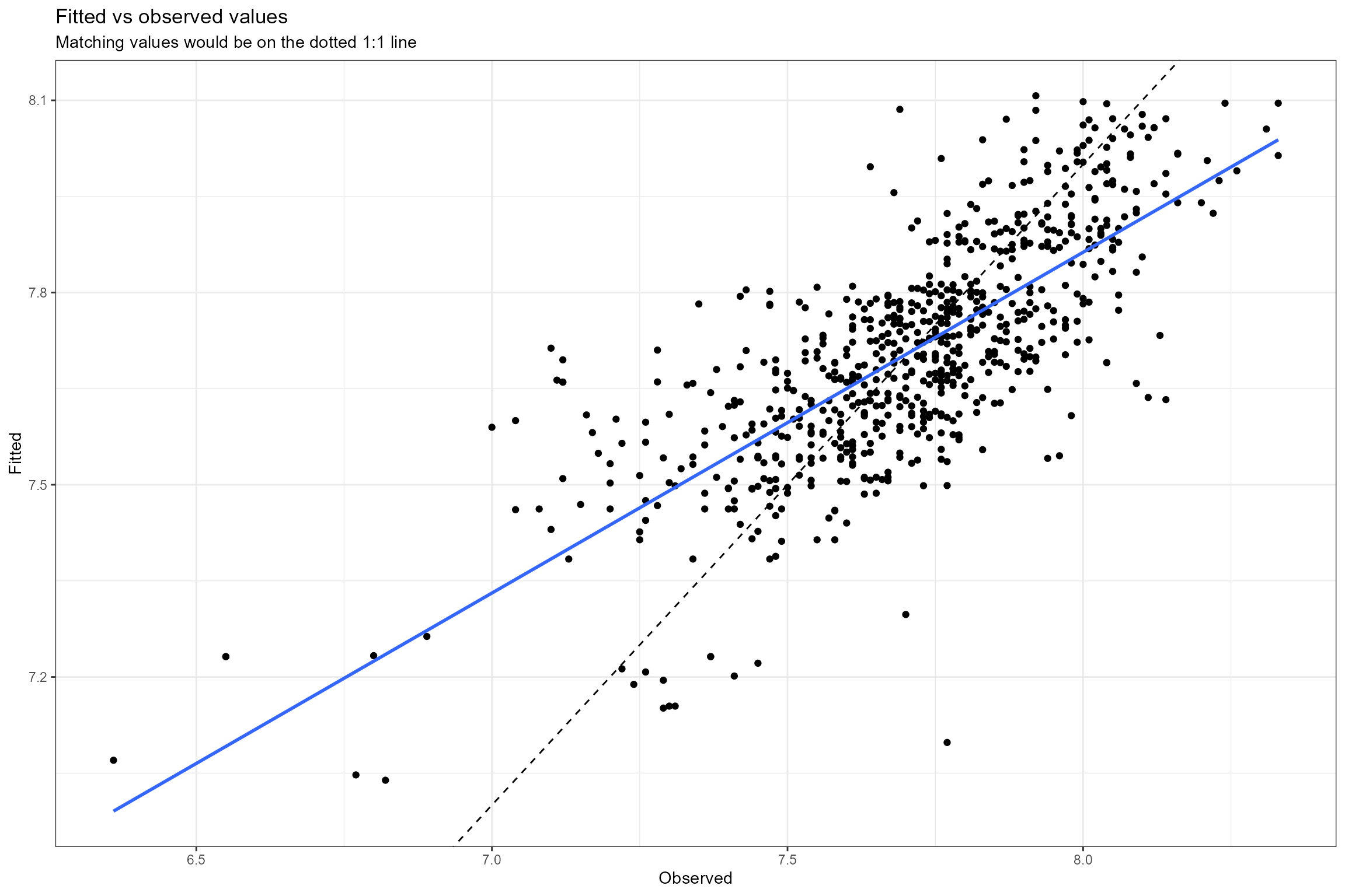
Fitted vs observed values. This plot shows the relationship between the fitted (predicted) and observed (true) values of the response variable. If the model fits the data well, the points should be clustered around the diagonal 1:1 line, which represents a perfect fit (fitted = observed). Here we can see the model provides a reasonably good fit to the data, but with a slight tendency to under-predict high RMHI values and over-predict low RMHI values (which is very common in regression modelling).

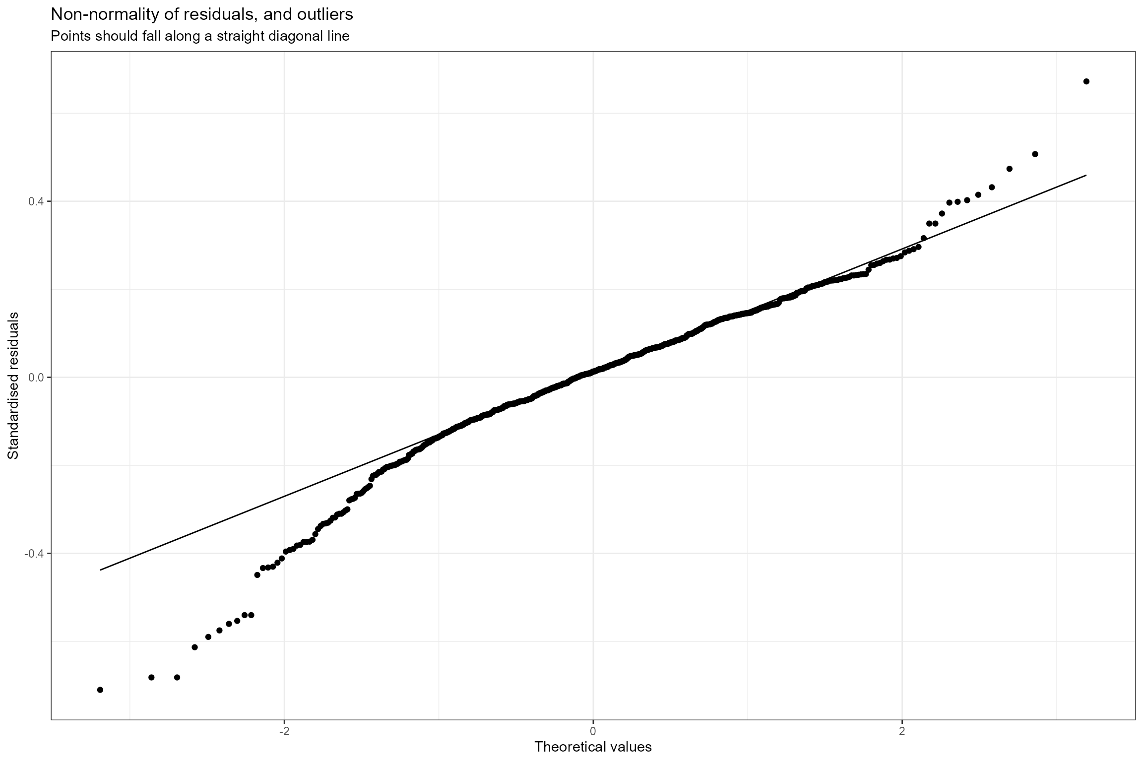
Normal probability plot. This is a graphical technique for verifying the assumption of a Normally-distributed error structure. The model residuals are plotted against a theoretical Normal distribution in such a way that the points should form an approximate straight line. Here we can see that the residuals conform closely to a Normal distribution, but with slightly more variance than expected.

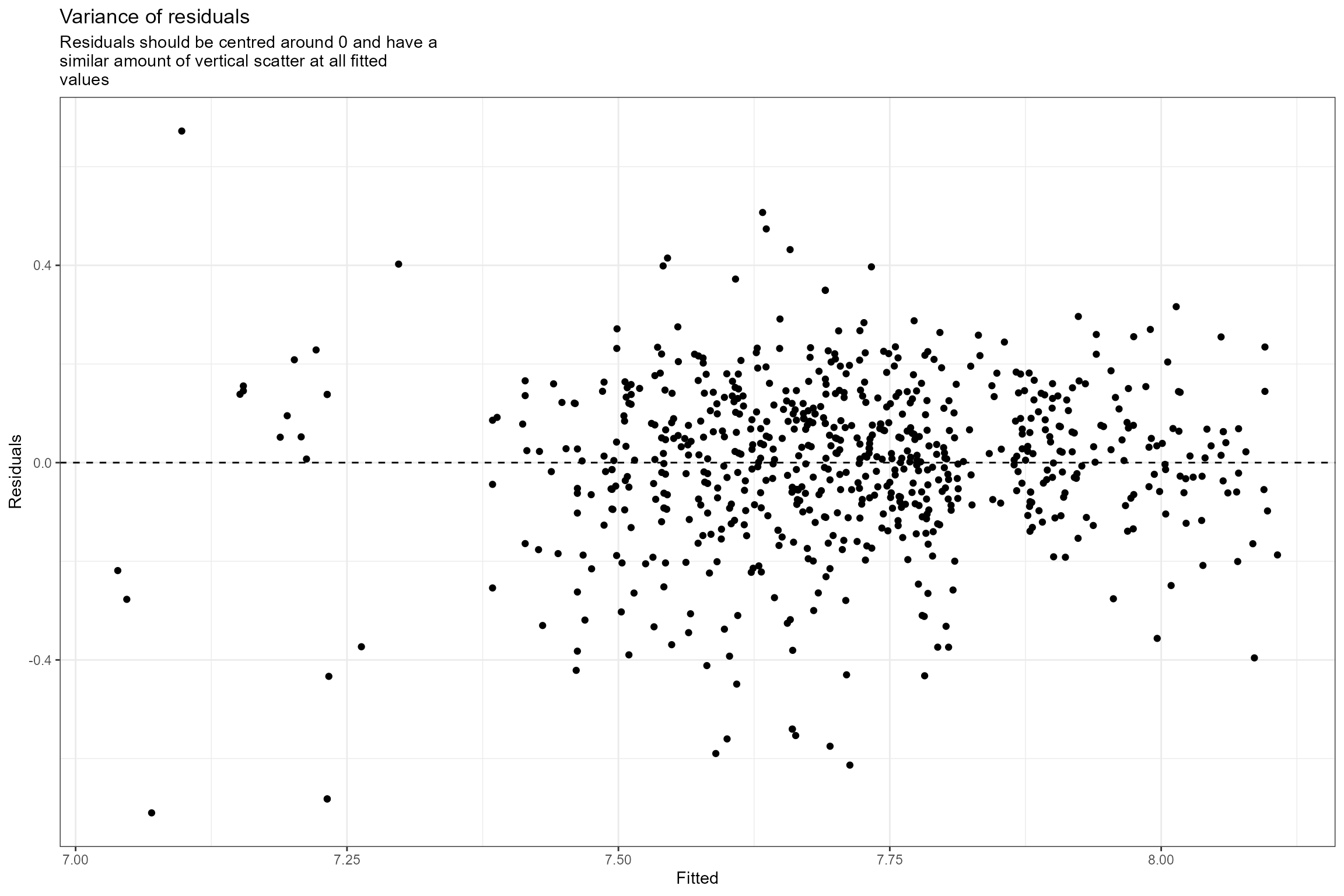
Residuals vs fitted values. This plot checks the assumption of homogeneous variances, which states that the error variance should be constant regardless of what value the response takes. Here we can see that the residuals have a similar amount of vertical scatter at all fitted values of the response, so this assumption is verified.

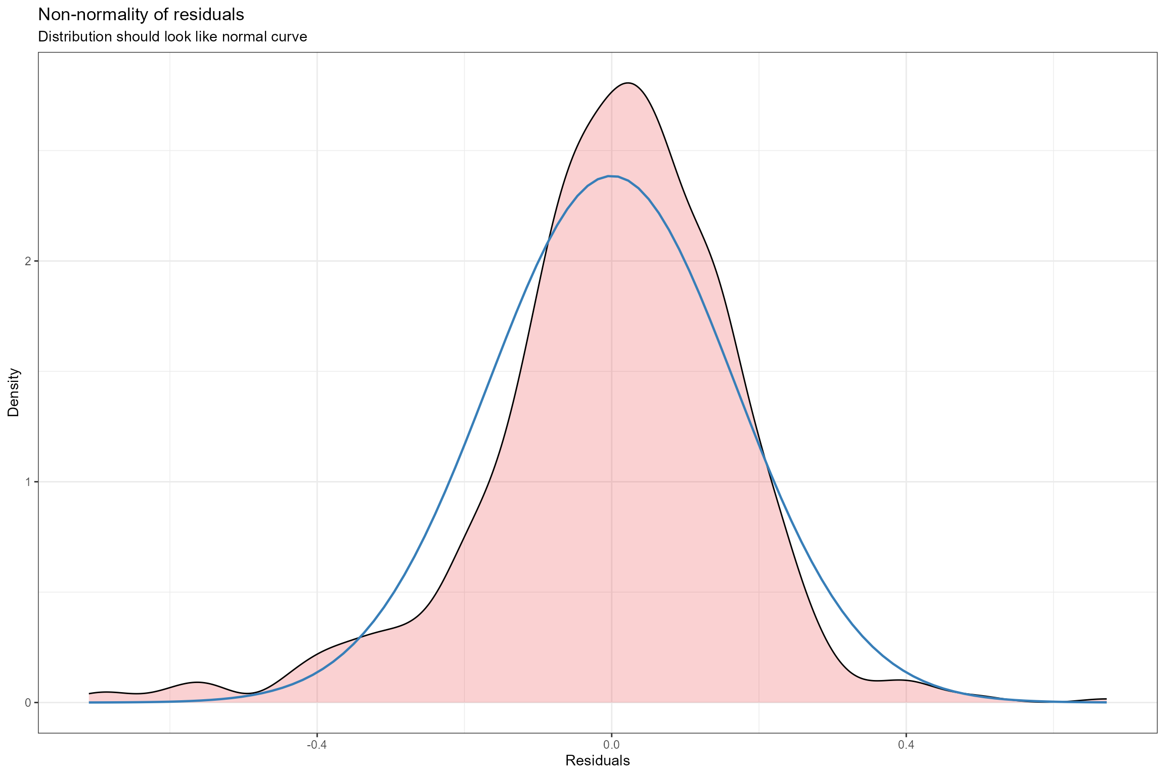
Histogram of residuals. This is an alternative to plot 2 for verifying the assumption of Normally-distributed errors. Here we can see that the probability distribution of the model residuals (shown by the pink shaded area) is fairly similar to a perfect Normal distribution (shown by the blue line).

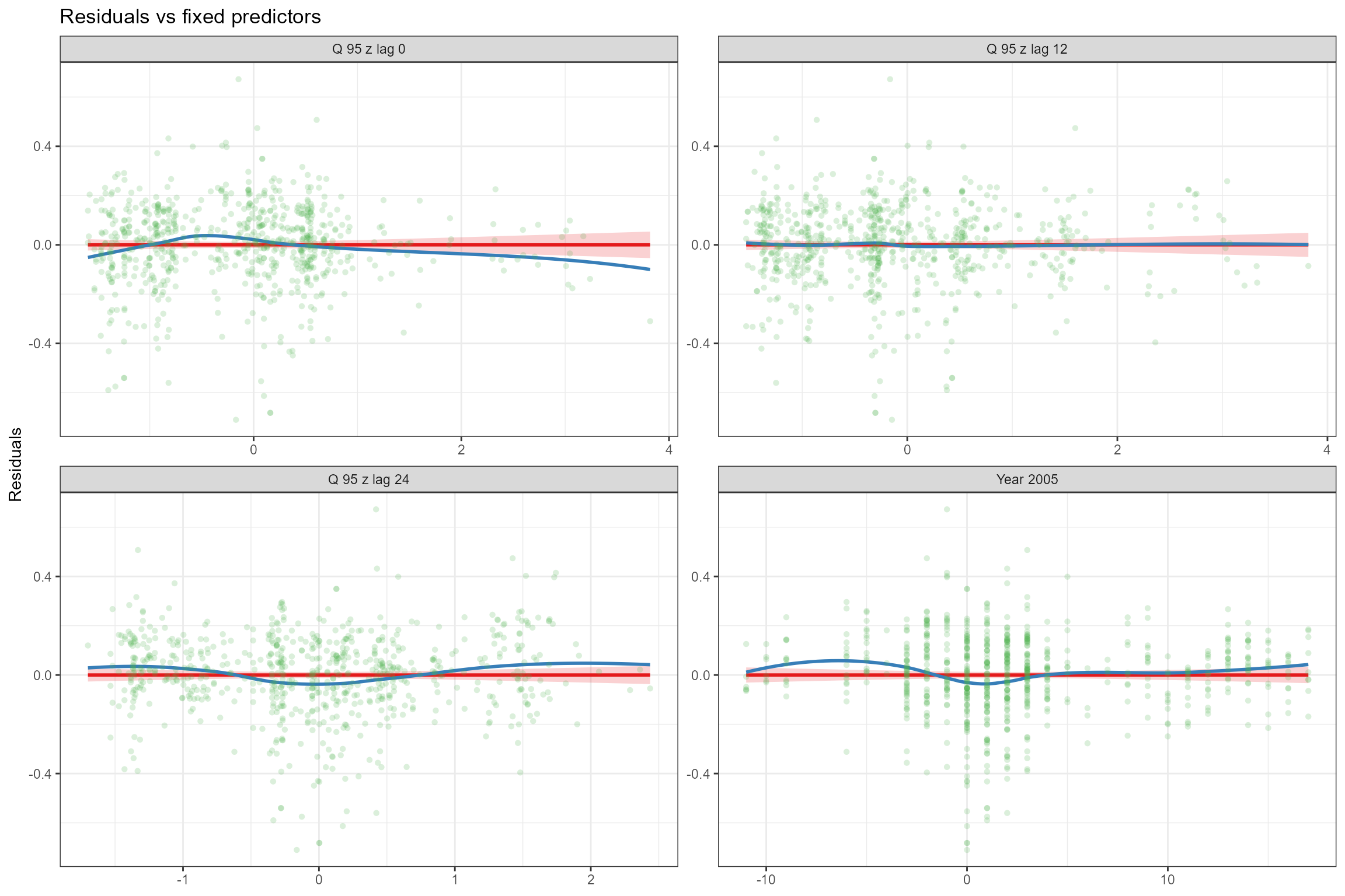
Residuals vs fixed predictors. To verify the assumption of linearity, the model’s residuals are plotted against each of the fixed predictors in turn. If the relationship between the response and each predictor is truly linear, then there should be no trend in the residuals. We can see that the linear (red) line fitted to the residuals is horizontal, indicating that that the strength of the linear effects has not been over- or under-estimated. And the loess-smoothed (blue) line is also close to horizontal, indicating that the relationships are approximately linear.

Other useful diagnostic plots for lmer models include:

Caterpillar plots, for visualising the random effects for each site. Our final model only has a random intercept, so the plot shows the estimated random effect (expressed as a deviation from the global intercept) for each site (biol_site_id). Sites coloured blue are those where, all else being equal, the mean RMHI is higher than average, and red sites have lower-than-average RMHI.

sjPlot::plot_model(model = cs3_mod_final, 
                   type = "re", 
                   facet.grid = FALSE, 
                   free.scale = FALSE, 
                   title = NULL, 
                   vline.color = "darkgrey")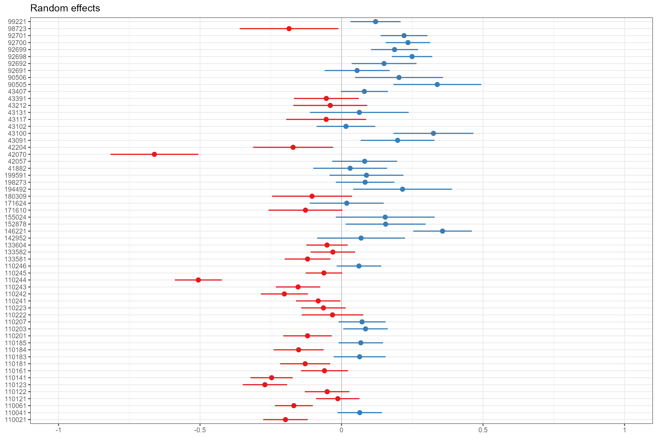

Partial effects plots, for visualising the modelled effect of each fixed predictor variable in turn when other continuous predictors are held constant at their mean values and factors are fixed at their reference level. This confirms the strong negative association between RMHI and Year_2005, and a positive effect of Q95z_lag0, Q95z_lag12 and Q95z_lag24.

sjPlot::plot_model(model = cs3_mod_final, 
                   type = "pred",
                   pred.type = "fe",
                   facet.grid = TRUE,
                   scales = "fixed", terms = "Year_2005")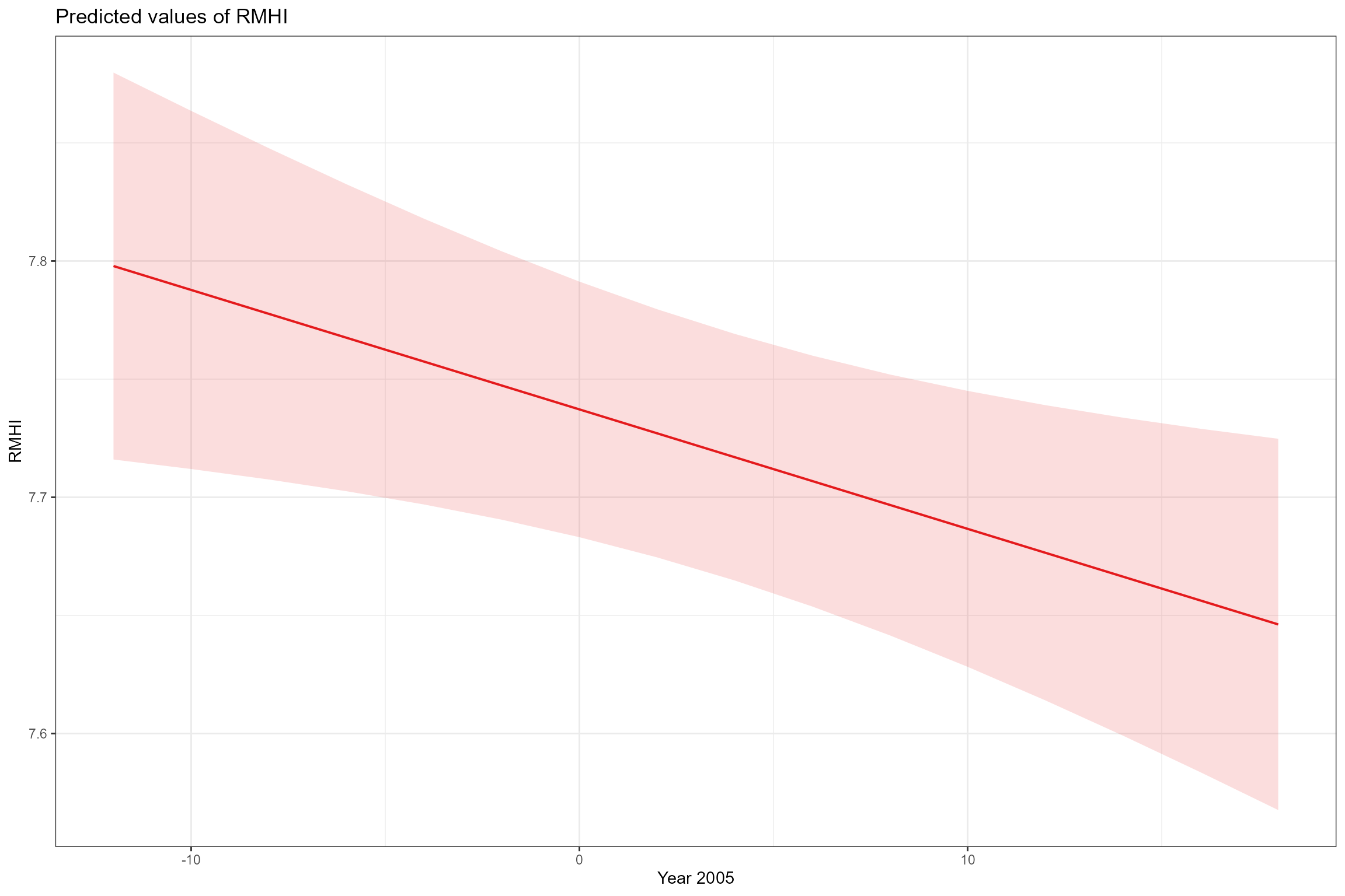

sjPlot::plot_model(model = cs3_mod_final, 
                   type = "pred",
                   pred.type = "fe",
                   facet.grid = TRUE,
                   scales = "fixed", terms = "Q95z_lag0")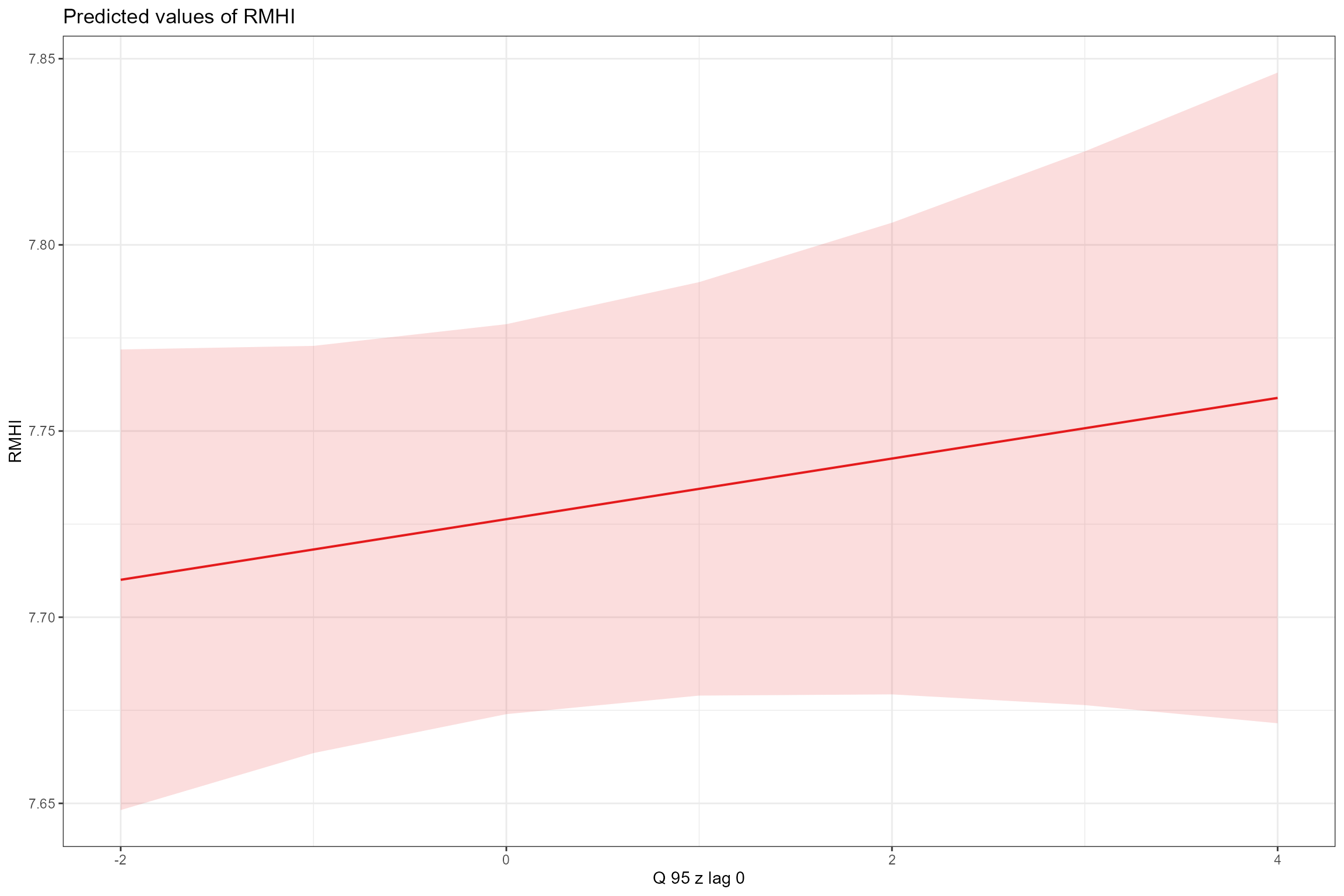

sjPlot::plot_model(model = cs3_mod_final, 
                   type = "pred",
                   pred.type = "fe",
                   facet.grid = TRUE,
                   scales = "fixed", terms = "Q95z_lag12")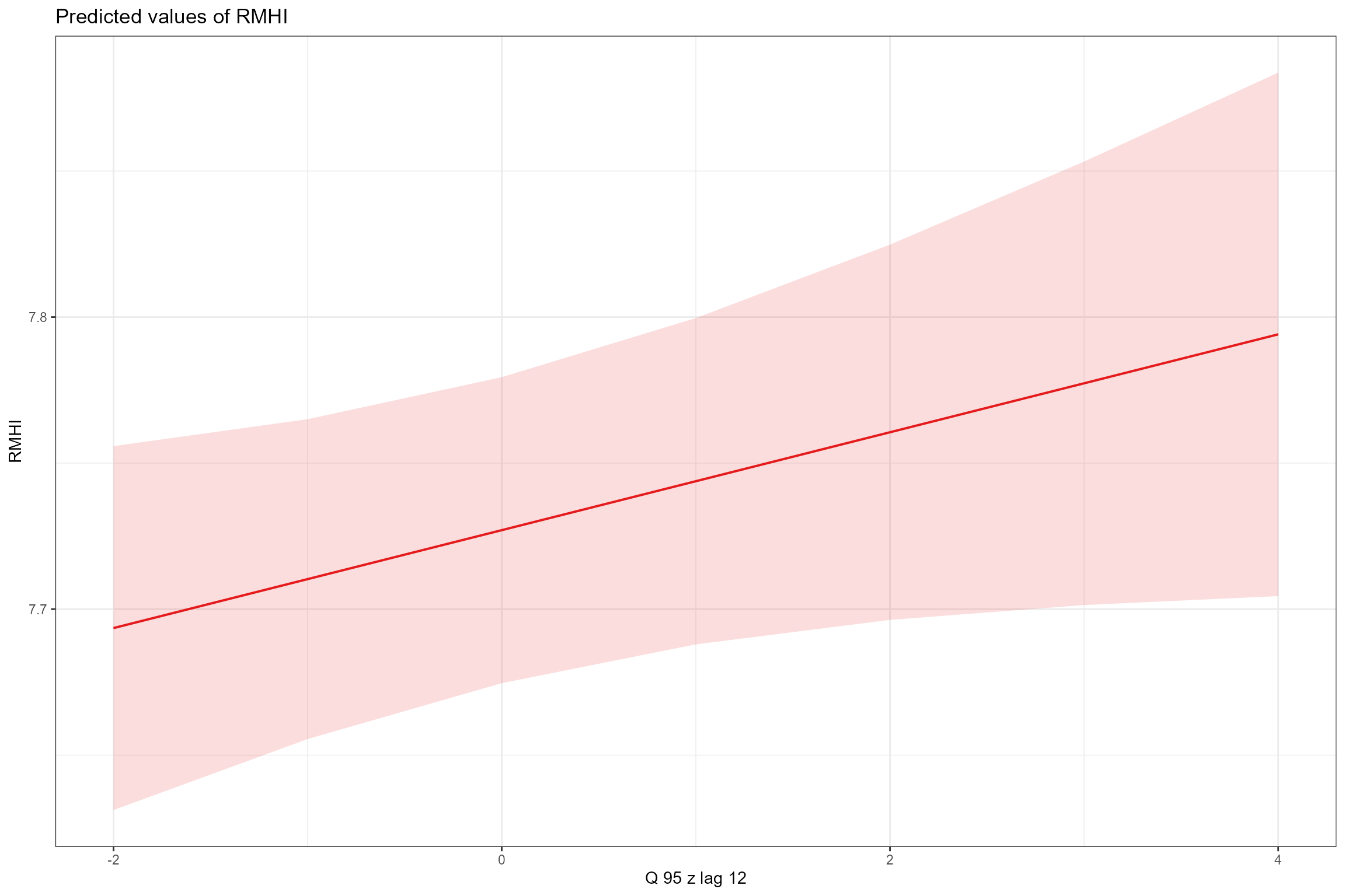

sjPlot::plot_model(model = cs3_mod_final, 
                   type = "pred",
                   pred.type = "fe",
                   facet.grid = TRUE,
                   scales = "fixed", terms = "Q95z_lag24")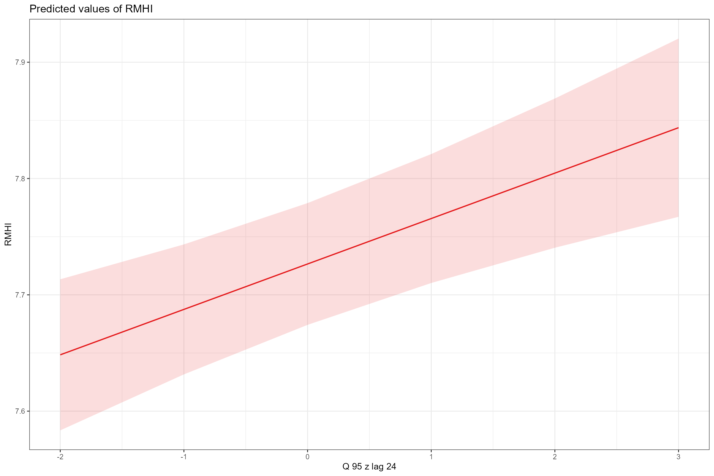

Scenario Analysis

Having calibrated a model using the flows experienced historically, we can use the final model to predict RMHI under alternative flow scenarios. For instance, we can make predictions of RMHI under naturalised flows; the difference between the predictions under historical and naturalised flows then provides a measure of how much abstraction pressure is affecting the macrophyte community.

The final model did not include the flow alteration variable LTQ95RFR (if it had, this variable could be fixed at 1 to represent an absence of flow alteration under a naturalised scenario), but it did include three flow history variables (Q95z_lag0, Q95z_lag12 and Q95z_lag24). Below we use the calc_flowstats function to calculate these Q95 flow statistics for naturalised flows. The function includes the facility to standardise the statistics for one flow scenario (specified via flow_col) using mean and standard deviation flow statistics from another scenario (specified via ref_col). For example, if flow_col = naturalised flows and ref_col = historical flows, then the resulting statistics can be input into a hydro-ecological model that has previously been calibrated using standardised historical flow statistics and used to make predictions of ecological status under naturalised flows.

# Use calc_flowstats() function to calculate Q95z (this may take a few minutes)
cs3_natural_scenario_flowstats <- hetoolkit::calc_flowstats(data = cs3_flowraw_wide,
                                           site_col= "flow_site_id",
                                           date_col= "Date",
                                           flow_col= "Naturalised",
                                           ref_col = "Historical",
                                           imputed_col= NULL,
                                           win_start = "1985-01-01",
                                           win_width = "1 year",
                                           win_step = "1 month",
                                           date_range = NULL)

# Extract data frame of time-varying flow statistics, and select only essential columns
cs3_natural_scenario_flowstats <- cs3_natural_scenario_flowstats[[1]] %>%
  dplyr::select(flow_site_id, win_no, start_date, end_date, Q95z_ref) %>% 
  dplyr::rename(Q95z = "Q95z_ref")

# Extract data from historical flow stats
cs3_historical_scenario_flowstats <- cs3_flowstats1 %>%
  dplyr::select(flow_site_id, win_no, start_date, end_date, Q95z)

Create the prediction data and join with the flow data

# Create a prediction data set
cs3_predict_biol_data <- expand.grid(
  biol_site_id = unique(cs3_biol_all$biol_site_id), 
  Year = seq(1995,2018)
  )

# Add year_2005 variable and a date variable 
cs3_predict_biol_data <- cs3_predict_biol_data %>%
  dplyr::mutate(Year_2005 = Year - 2005) %>%
  dplyr::mutate(date = as.Date(paste0(Year, "-08-15"), format = "%Y-%m-%d"))

# Join flow data
cs3_natural_he <- hetoolkit::join_he(biol_data = cs3_predict_biol_data,
                                     flow_stats = cs3_natural_scenario_flowstats,
                                     mapping = cs3_metadata,
                                     lags = c(0, 12, 24),
                                     method = "A",
                                     join_type = "add_flows")

cs3_historical_he <- hetoolkit::join_he(biol_data = cs3_predict_biol_data,
                                        flow_stats =
                                          cs3_historical_scenario_flowstats,
                                        mapping = cs3_metadata,
                                        lags = c(0,12,24),
                                        method = "A",
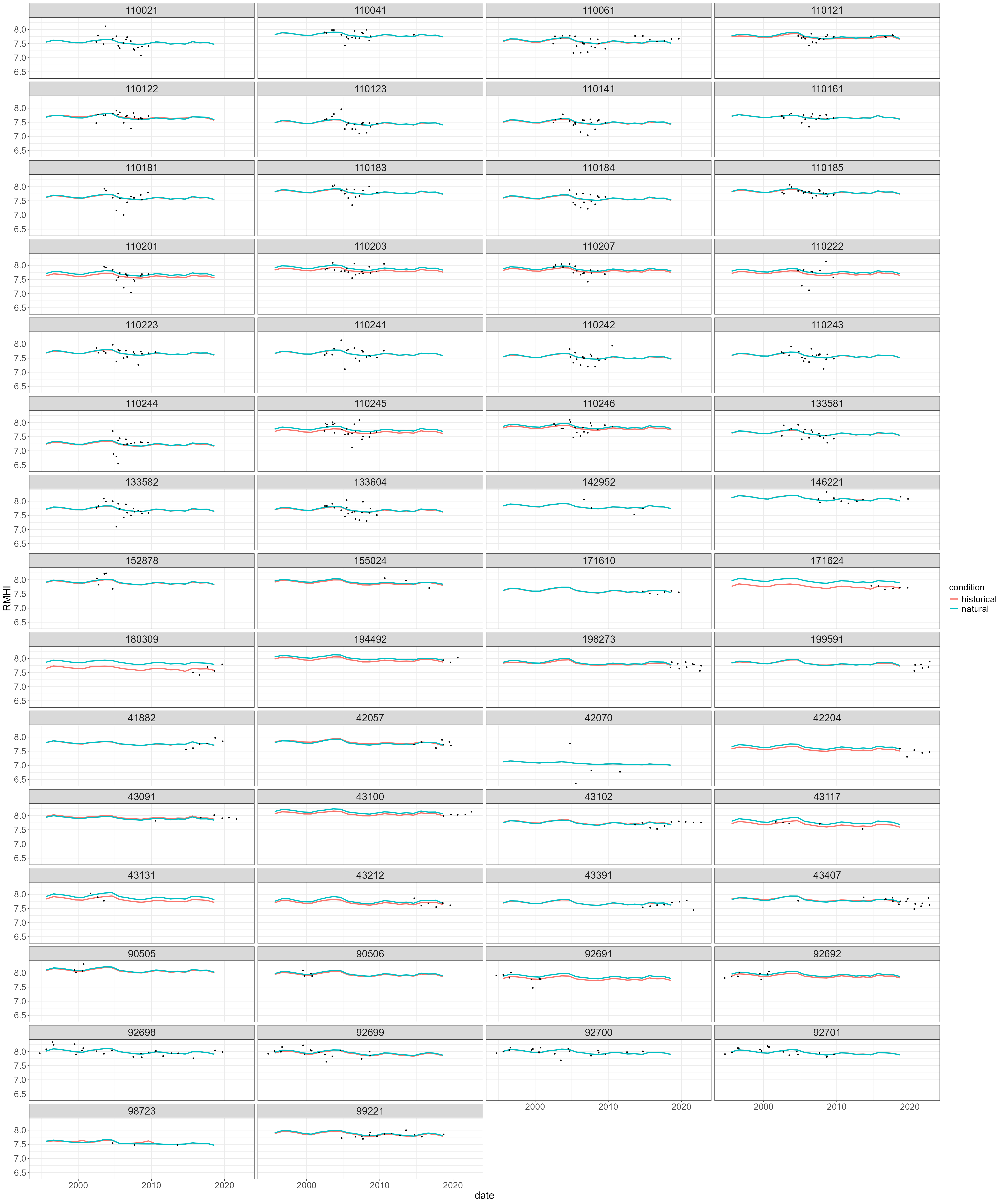
                                        join_type = "add_flows")

Now we can use the predict function to predict RMHI under both the naturalised and historical scenarios, and plot the results. We can see how the “historical” line describes the patterns in the historical data (the black points), and interpret the difference between the historical and naturalised scenarios as the effect of flow alteration. In this example, the historic and naturalised predictions are broadly similar, though with some evidence that flow alteration is altering RMHI scores at a subset of sites.

# Make predictions
cs3_natural_he$predict <- predict(cs3_mod_final, newdata = cs3_natural_he)
cs3_historical_he$predict <- predict(cs3_mod_final, newdata = cs3_historical_he)

# Create a data frame with the predicted values, biol_site_id, date and scenario (natural or historical), 
# ready for plotting
cs3_predicted_data <- rbind(
  data.frame(value = cs3_natural_he$predict, condition = "natural", 
             biol_site_id = cs3_natural_he$biol_site_id, date = cs3_natural_he$date),
  data.frame(value = cs3_historical_he$predict, condition = "historical", 
             biol_site_id= cs3_historical_he$biol_site_id, date = cs3_historical_he$date)
)

# Plot the predictions, with the true (measured) values as points for reference.
ggplot(cs3_predicted_data, aes(x = date, y = value, color = condition)) +
  geom_line(size = 1) +
  geom_point(data = cs3_biol_all, aes(x = date, y = RMHI, color = "measured"), size = 0.7, colour = "black") +
  facet_wrap(~ biol_site_id, ncol = 4) +
  labs(y = "RMHI") +
  theme(axis.title = element_text(size=18), axis.text = element_text(size = 16),
  strip.text = element_text(size=18), legend.text = element_text(size=16), 
  legend.title = element_text(size = 16))

Environment Agency / APEM Ltd

23 January, 2025

Introduction

Set-up

Metadata file

Macrophyte data

Import macrophyte data

Visualise macrophyte data

Water quality data

Import data

Explore data

Summarise data

Flow data

Import data

Visualise data

Calculate flow statistics

Flow alteration metric

Flow history metric

Join hydrological and ecological data

Modelling

Assess coverage of historical flow conditions

Data preparation

Model calibration

Model interpretation

Model diagnostics

Scenario Analysis